


Most real-world classification issues are imbalanced. Fraud, illness, churn, and defects are uncommon by nature. Commonplace classifiers chase accuracy, so that they quietly ignore the very class you care about. For years, SMOTE was the reflex repair that everybody reached for first.
However SMOTE typically fails on the messy, high-dimensional information that manufacturing programs truly see. This information goes past SMOTE. You’ll study cost-sensitive studying, fashionable loss capabilities, balanced ensembles, anomaly detection, and the metrics that expose what actually works.
What Is Class Imbalance?
Class imbalance describes a skewed distribution between the goal lessons you wish to predict. The smaller group is the minority class, and the bigger group is almost all class. We normally categorical the skew as an imbalance ratio, resembling 100:1. A ratio of 100:1 means one uncommon case seems for each hundred frequent ones.
The minority class is nearly at all times the one with enterprise worth. Fraudulent transactions, malignant tumors, and churning prospects are uncommon however costly to overlook. So the price of errors is uneven, and that asymmetry ought to drive each modeling selection you make.
The place Imbalance Reveals Up in Observe
Imbalance is the rule, not the exception, throughout utilized machine studying. The uncommon class is the sign, and the frequent class is the background noise. The next domains all share this construction, and every one rewards cautious dealing with of the minority class.
- Fraud detection: Fraudulent transactions typically make up properly underneath 1% of all exercise. A mannequin should flag them with out drowning analysts in false alarms.
- Medical analysis: Most screened sufferers are wholesome, so optimistic circumstances are uncommon. Lacking a real optimistic might be life-threatening, which raises the price of false negatives.
- Churn prediction: Solely a small fraction of consumers cancel in any given month. Catching them early allows focused retention affords.
- Anomaly and fault detection: Machines run usually more often than not. Failures are uncommon, sudden, and really expensive to miss.
- Uncommon-event forecasting: Pure disasters, gear breakdowns, and safety breaches are rare however high-impact occasions value predicting.
Why Accuracy Is a Deceptive Metric
Accuracy measures the share of right predictions throughout all lessons equally. That sounds cheap till one class dominates the dataset. With a 98% majority class, a mannequin can hit 98% accuracy by predicting nothing helpful. It merely labels each case as the bulk and by no means finds the uncommon occasion.
This is the reason accuracy lies on imbalanced information. A excessive rating can conceal a mannequin that’s utterly blind to the minority class. You want metrics that concentrate on the uncommon class, resembling precision, recall, and PR-AUC. We’ll return to these metrics intimately later.
Setting Up the Playground: Dataset, Setting, and Baseline
Earlier than evaluating methods, we want one constant dataset and a transparent baseline. A shared playground lets us decide every methodology on equal footing. We’ll construct an artificial fraud-like dataset with heavy imbalance. Then we are going to practice a naive classifier to point out precisely how accuracy misleads.
The Dataset We’ll Use All through
We generate a binary dataset with 20,000 samples and a roughly 2% minority class. This mimics a practical fraud or rare-event situation with no need non-public information. Utilizing artificial information retains the examples reproducible on any machine. You may swap in your personal dataset later with virtually no code adjustments.
Setting and Libraries
The examples depend on a small, commonplace stack from the Python ecosystem. Every library performs a selected function within the imbalanced-learning workflow. Set up them with pip earlier than operating any of the code beneath.
scikit-learn: Core fashions, metrics, splitting, and the pipeline equipment.- i
mbalanced-learn(imblearn): Resamplers like SMOTE plus balanced ensembles resembling Balanced Random Forest. XGBoost/LightGBM: Gradient boosting with built-in assist for sophistication weighting and customized targets.
pip set up scikit-learn imbalanced-learn xgboostCode Demo: Loading the Knowledge and Inspecting the Imbalance
First, we create the dataset and examine its class distribution. All the time have a look at the uncooked counts earlier than modeling something. We additionally cut up the information with stratification to protect the imbalance ratio. Stratified splitting retains the minority share constant throughout practice and check units.
import numpy as np
from collections import Counter

from sklearn.datasets import make_classification
from sklearn.model_selection import train_test_split


ification
from sklearn.model_selection import train_test_split


RANDOM_STATE = 42

# Shared "playground" dataset: a ~2% fraud-like minority class
X, y = make_classification(
    n_samples=20000,
    n_features=20,
    n_informative=6,
    n_redundant=4,
    n_clusters_per_class=2,
    weights=[0.98, 0.02],
    class_sep=0.8,
    flip_y=0.01,
    random_state=RANDOM_STATE,
)

print("Whole samples:", X.form[0], "| Options:", X.form[1])
print("Class distribution:", dict(Counter(y)))

neg, pos = Counter(y)[0], Counter(y)[1]

print(f"Minority class share: {pos / (pos + neg):.2%}")
print(f"Imbalance ratio (majority:minority) = {neg / pos:.0f} : 1")

X_train, X_test, y_train, y_test = train_test_split(
    X,
    y,
    test_size=0.25,
    stratify=y,
    random_state=RANDOM_STATE,
)

print("Practice class counts:", dict(Counter(y_train)))
print("Take a look at class counts:", dict(Counter(y_test)))
Output:
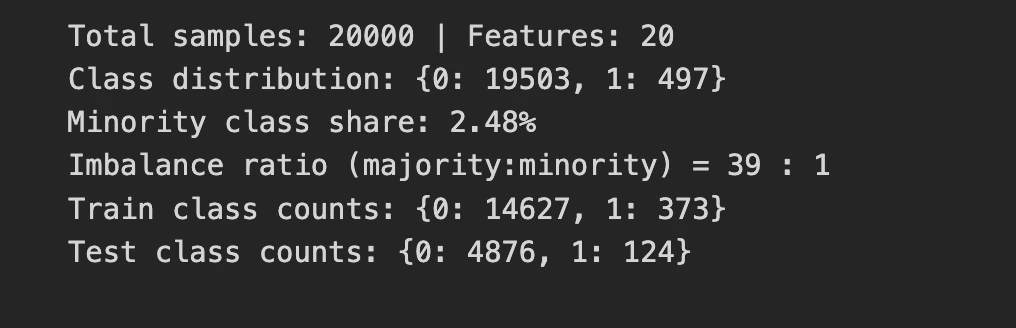
Code Demo: A Naive Baseline Classifier
Now we practice a plain logistic regression with no imbalance dealing with. We then evaluate its accuracy in opposition to its recall on the minority class. The hole between these two numbers is the guts of the issue. Watch how a excessive accuracy rating hides a near-useless mannequin.
from sklearn.linear_model import LogisticRegression
from sklearn.metrics import (
    accuracy_score,
    balanced_accuracy_score,
    confusion_matrix,
    classification_report,
)


clf = LogisticRegression(max_iter=2000)

clf.match(X_train, y_train)
y_pred = clf.predict(X_test)

print("Accuracy         :", spherical(accuracy_score(y_test, y_pred), 4))
print("Balanced accuracy:", spherical(balanced_accuracy_score(y_test, y_pred), 4))
print("Confusion matrix:n", confusion_matrix(y_test, y_pred))
print(classification_report(y_test, y_pred, digits=3))


# A mannequin that predicts EVERYTHING as the bulk class
dummy = np.zeros_like(y_test)

print(
    "Predict-all-majority accuracy:",
    spherical(accuracy_score(y_test, dummy), 4),
)
Output:
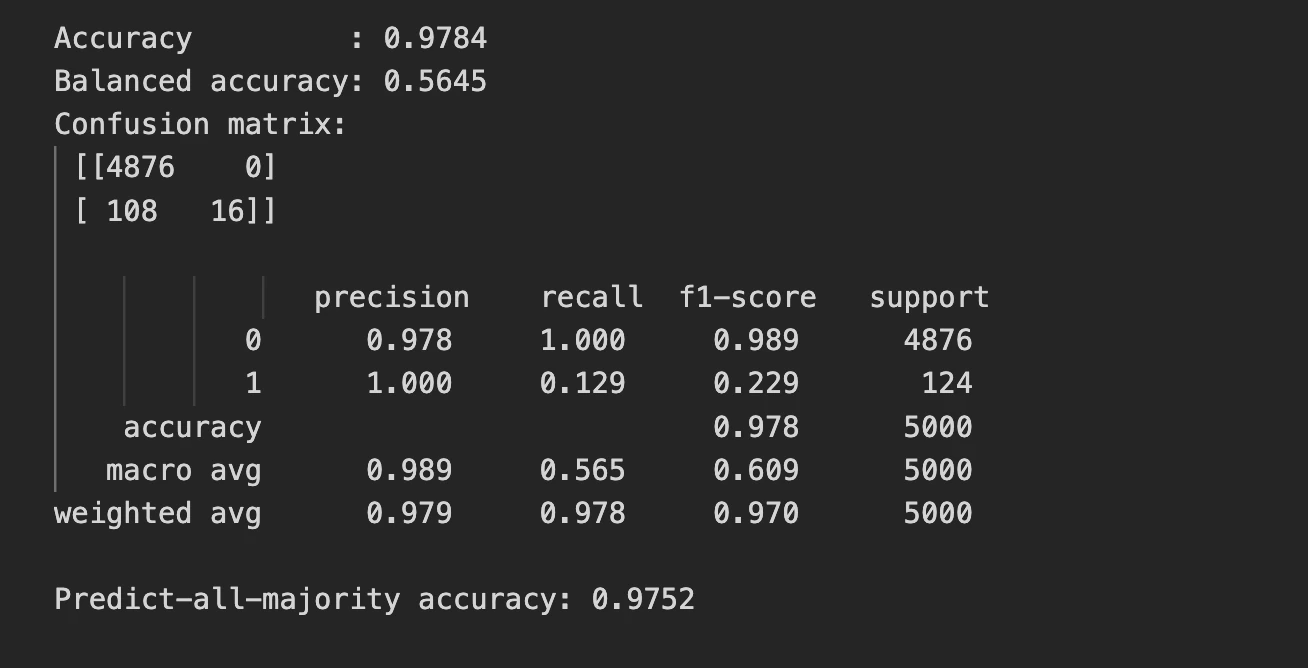
The mannequin scores 97.8% accuracy but catches solely 12.9% of fraud circumstances. A mannequin that blindly predicts “not fraud” scores 97.5% accuracy. So our skilled mannequin barely beats doing nothing in any respect. This single consequence motivates each approach in the remainder of the information.
A Fast Refresher on SMOTE and Its Variants
SMOTE is probably the most well-known reply to class imbalance, so it deserves a good abstract. It tackles imbalance on the information stage by inventing new minority examples. Understanding the way it works explains each its enchantment and its failure modes. Let’s assessment the mechanism earlier than we stress-test it.
How SMOTE Works
SMOTE stands for Artificial Minority Over-sampling Method. As an alternative of copying minority factors, it creates new ones by interpolation. It picks a minority pattern, finds its nearest minority neighbors, and attracts a brand new level between them. This fills out the minority area fairly than simply duplicating present rows.
The aim is a extra balanced coaching set with out easy over-duplication. In concept, the classifier then sees a richer minority distribution. In follow, the standard of these artificial factors relies upon closely on the information. That dependence is precisely the place SMOTE begins to battle.
In style Extensions
Researchers constructed many SMOTE variants to patch its weaknesses. Each adjustments how or the place artificial samples get created. The most typical variants can be found straight in imbalanced-learn.
- Borderline-SMOTE: Generates samples solely close to the choice boundary, the place errors are most certainly.
- ADASYN: Creates extra artificial factors for minority samples which might be tougher to categorise.
- SMOTE-NC: Handles datasets that blend steady and categorical options.
- SVM-SMOTE: Makes use of a assist vector machine to search out good areas for brand spanking new samples.
- SMOTE-ENN and SMOTE-Tomek: Mix oversampling with cleansing steps that take away noisy or overlapping factors.
Code Demo: SMOTE in Motion
Right here we apply SMOTE inside a correct pipeline and examine the outcomes. We resample solely the coaching information, by no means the check information. Discover the before-and-after class counts and the shift in scores. Pay shut consideration to what occurs to precision and recall.
from collections import Counter

from sklearn.linear_model import LogisticRegression
from sklearn.metrics import classification_report, average_precision_score
from imblearn.over_sampling import SMOTE
from imblearn.pipeline import Pipeline


print("Earlier than SMOTE:", dict(Counter(y_train)))

X_res, y_res = SMOTE(random_state=RANDOM_STATE).fit_resample(
    X_train,
    y_train,
)

print("After SMOTE:", dict(Counter(y_res)))


# Right utilization: SMOTE inside a pipeline, so it solely touches coaching folds
pipe = Pipeline(
    [
        ("smote", SMOTE(random_state=RANDOM_STATE)),
        ("clf", LogisticRegression(max_iter=2000)),
    ]
)

pipe.match(X_train, y_train)

y_pred = pipe.predict(X_test)
y_proba = pipe.predict_proba(X_test)[:, 1]

print(classification_report(y_test, y_pred, digits=3))
print("PR-AUC:", spherical(average_precision_score(y_test, y_proba), 4))
Output:
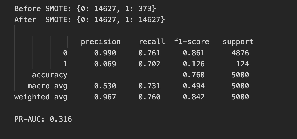
SMOTE lifts recall from 12.9% to 70.2%, which seems like a win. However precision collapses from 100% to simply 6.9% within the course of. The mannequin now flags enormous numbers of legit circumstances as fraud. This trade-off is the core pressure we should handle fastidiously.
Why SMOTE Typically Fails within the Actual World
SMOTE works properly in tidy, low-dimensional, well-separated datasets. Manufacturing information is never tidy, low-dimensional, or well-separated. The approach makes a number of assumptions that actual datasets routinely violate. Listed below are the failure modes you’ll truly encounter.
Synthesizing Noise and Amplifying Overlap
SMOTE interpolates between minority factors with out checking class boundaries. When minority and majority lessons overlap, it generates factors inside enemy territory. These artificial samples blur the boundary as a substitute of sharpening it. The classifier then learns a fuzzier, much less dependable determination rule.
Poor Efficiency in Excessive Dimensions
Nearest-neighbor distances turn into unreliable because the variety of options grows. That is the curse of dimensionality, and SMOTE relies upon solely on neighbors. In excessive dimensions, “close by” factors might not be meaningfully related. The interpolated samples then land in areas that make little sense.
The Curse of Categorical and Combined Knowledge
Plain SMOTE assumes steady options so it might probably interpolate easily. Categorical options break that assumption as a result of averaging classes is meaningless. The midway level between “bank card” and “wire switch” merely doesn’t exist. You want SMOTE-NC or encoding methods, and even these have sharp limits.
Knowledge Leakage When Oversampling Earlier than Splitting
The only most typical SMOTE mistake is resampling earlier than the train-test cut up. Artificial factors then leak info from the check set into coaching. Your validation scores look improbable and your manufacturing scores crater. All the time resample inside a pipeline, utilized per fold, after splitting.
It Optimizes the Incorrect Goal
SMOTE rebalances the information, however stability is just not the precise enterprise aim. You normally need a good rating of threat, not a 50-50 class cut up. Typically the mannequin already ranks properly and easily wants a greater threshold. Resampling can disturb a superb rating whereas chasing synthetic stability.
Code Demo: Watching SMOTE Break
This demo exhibits leakage inflating scores to absurd ranges. We cross-validate two methods: oversampling earlier than splitting and oversampling contained in the pipeline. The distinction in F1 rating is dramatic and sobering. It proves why pipeline self-discipline is non-negotiable.
from sklearn.model_selection import cross_val_score, StratifiedKFold
from sklearn.linear_model import LogisticRegression
from imblearn.over_sampling import SMOTE
from imblearn.pipeline import Pipeline


cv = StratifiedKFold(
    n_splits=5,
    shuffle=True,
    random_state=RANDOM_STATE,
)

# WRONG: oversample the entire dataset, THEN cross-validate
X_leak, y_leak = SMOTE(random_state=RANDOM_STATE).fit_resample(X, y)

leaky = cross_val_score(
    LogisticRegression(max_iter=2000),
    X_leak,
    y_leak,
    cv=cv,
    scoring="f1",
)

print("Leaky CV F1 (SMOTE earlier than cut up):", spherical(leaky.imply(), 3))


# RIGHT: SMOTE contained in the pipeline, utilized to coaching folds solely
pipe = Pipeline(
    [
        ("smote", SMOTE(random_state=RANDOM_STATE)),
        ("clf", LogisticRegression(max_iter=2000)),
    ]
)

trustworthy = cross_val_score(
    pipe,
    X,
    y,
    cv=cv,
    scoring="f1",
)

print("Sincere CV F1 (SMOTE inside pipe):", spherical(trustworthy.imply(), 3))
Output:

The leaky setup experiences an F1 of 0.748, which might thrill any stakeholder. The trustworthy pipeline experiences 0.127, which is the painful fact. That’s almost a six-fold inflation from one frequent mistake. All the time hold your resampling sealed contained in the cross-validation loop.
Rethinking the Method: 4 Ranges of Intervention
Cease pondering of imbalance as an information drawback with one repair. Consider it as a system with 4 factors the place you may intervene. Every stage affords totally different instruments and totally different trade-offs. Selecting the best stage issues greater than selecting the trendiest algorithm.
Knowledge-Stage Strategies
Knowledge-level strategies change the coaching distribution earlier than studying begins. They embody oversampling, undersampling, and hybrid approaches like SMOTE-ENN. These strategies are model-agnostic and simple to bolt onto any pipeline. Nonetheless, they threat discarding helpful information or inventing deceptive samples.
Algorithm-Stage Strategies
Algorithm-level strategies go away the information alone and alter the learner as a substitute. They reshape the loss perform so minority errors price extra. Class weights, price matrices, and focal loss all dwell at this stage. These strategies typically beat resampling whereas avoiding synthetic-data artifacts.
Ensemble-Stage Strategies
Ensemble-level strategies mix many fashions skilled on balanced subsamples. Every base learner sees a good struggle between the lessons. The ensemble then aggregates their votes into a robust last prediction. Balanced Random Forest and RUSBoost are the standout examples right here.
Choice-Stage Strategies
Output-level strategies alter the choice after the mannequin produces scores. The traditional transfer is tuning the chance threshold away from 0.5. You may also calibrate chances to make them reliable. These strategies are low cost, highly effective, and shamefully underused in follow.
Methods to Determine Which Stage to Goal First
Begin on the determination stage as a result of it’s the most cost-effective experiment. Tune the brink on a robust baseline earlier than touching the information. Transfer to algorithm-level weighting subsequent, because it provides no artificial noise. Attain for resampling or ensembles solely when these less complicated steps fall quick.
Algorithm-Stage Methods That Really Work
Algorithm-level methods repair imbalance by altering how the mannequin learns. They make the minority class costly to disregard. Crucially, they keep away from the synthetic-data dangers that plague SMOTE. These strategies are sometimes the highest-value first transfer you can also make.
Price-Delicate Studying
Price-sensitive studying tells the mannequin that some errors harm greater than others. A missed fraud ought to price greater than a false alarm. We encode this asymmetry straight into the coaching goal. The mannequin then learns a boundary that respects the true prices.
Class Weights
Most scikit-learn classifiers settle for a class_weight parameter for this function. Setting it to “balanced” weights every class inversely to its frequency. The minority class will get extra affect on the loss with none new information. That is the only cost-sensitive methodology, and it really works remarkably properly.
Price Matrices
A price matrix assigns a selected penalty to every sort of error. False negatives and false positives can carry very totally different costs. This strategy shines when the true enterprise price of errors. You then optimize anticipated price fairly than a generic statistical metric.
Code Demo: Class Weights vs. Resampling
Right here we evaluate a plain mannequin, a class-weighted mannequin, and a SMOTE mannequin. We observe precision, recall, F1, and PR-AUC for every. The consequence reveals one thing refined about what these strategies truly do. Watch the PR-AUC column particularly carefully.
from sklearn.linear_model import LogisticRegression
from sklearn.metrics import (
    precision_score,
    recall_score,
    f1_score,
    average_precision_score,
)
from imblearn.over_sampling import SMOTE
from imblearn.pipeline import Pipeline


def report(identify, mannequin):
    mannequin.match(X_train, y_train)

    p = mannequin.predict(X_test)
    pr = mannequin.predict_proba(X_test)[:, 1]

    print(
        f"{identify:<28} "
        f"P={precision_score(y_test, p):.3f} "
        f"R={recall_score(y_test, p):.3f} "
        f"F1={f1_score(y_test, p):.3f} "
        f"PR-AUC={average_precision_score(y_test, pr):.3f}"
    )


report(
    "Plain LogisticRegression",
    LogisticRegression(max_iter=2000),
)

report(
    "class_weight="balanced"",
    LogisticRegression(max_iter=2000, class_weight="balanced"),
)

report(
    "SMOTE + LogisticRegression",
    Pipeline(
        [
            ("s", SMOTE(random_state=RANDOM_STATE)),
            ("c", LogisticRegression(max_iter=2000)),
        ]
    ),
)
Output:

Class weights and SMOTE land in virtually precisely the identical place. Each shift the choice boundary towards increased recall and decrease precision. But the plain mannequin has the best PR-AUC of all three. Which means its underlying rating is greatest; it simply wants a greater threshold. This can be a important clue that resampling is usually pointless.
Trendy Loss Features for Imbalance
Loss capabilities might be redesigned to focus studying on onerous, uncommon circumstances. These fashionable losses emerged largely from laptop imaginative and prescient analysis. They now apply properly to tabular and deep-learning imbalance issues. Every reshapes the gradient to cease straightforward majority circumstances from dominating.
- Focal Loss: Down-weights straightforward, well-classified examples so the mannequin focuses on onerous ones.
- Class-Balanced Loss: Reweights lessons utilizing the efficient variety of samples, not uncooked counts.
- LDAM Loss: Enforces bigger margins for minority lessons to enhance generalization.
- Uneven Loss: Treats optimistic and adverse errors in a different way, which fits multi-label imbalance.
Code Demo: Focal Loss in Observe
We implement focal loss as a customized goal for XGBoost. The target down-weights assured, right predictions mechanically. We then evaluate it in opposition to commonplace log loss on the identical information. Focal loss ought to sharpen the mannequin’s concentrate on the uncommon class.
import numpy as np
import xgboost as xgb

from sklearn.metrics import (
    precision_score,
    recall_score,
    f1_score,
    average_precision_score,
)


def _focal_grad(z, y, gamma, alpha):
    p = np.clip(1.0 / (1.0 + np.exp(-z)), 1e-6, 1 - 1e-6)

    at = np.the place(y == 1, alpha, 1 - alpha)  # class-balancing weight
    pt = np.the place(y == 1, p, 1 - p)  # prob assigned to true class
    s = np.the place(y == 1, 1.0, -1.0)

    return at * s * (1 - pt) ** gamma * (
        gamma * pt * np.log(pt) - (1 - pt)
    )


def focal_binary_obj(gamma=2.0, alpha=0.75):
    def obj(y_pred, dtrain):
        y = dtrain.get_label()

        grad = _focal_grad(y_pred, y, gamma, alpha)

        eps = 1e-4  # hessian through central distinction
        hess = (
            _focal_grad(y_pred + eps, y, gamma, alpha)
            - _focal_grad(y_pred - eps, y, gamma, alpha)
        ) / (2 * eps)

        return grad, np.most(hess, 1e-6)

    return obj


dtr = xgb.DMatrix(X_train, label=y_train)
dte = xgb.DMatrix(X_test, label=y_test)

params = {
    "max_depth": 4,
    "eta": 0.1,
    "seed": RANDOM_STATE,
    "verbosity": 0,
}

m_std = xgb.practice(
    {**params, "goal": "binary:logistic"},
    dtr,
    num_boost_round=300,
)

m_fl = xgb.practice(
    params,
    dtr,
    num_boost_round=300,
    obj=focal_binary_obj(2.0, 0.75),
)

p_std = m_std.predict(dte)

# Focal loss outputs uncooked margins
p_fl = 1 / (1 + np.exp(-m_fl.predict(dte)))

for identify, prob in [
    ("XGBoost (logloss)", p_std),
    ("XGBoost (focal loss)", p_fl),
]:
    pred = (prob >= 0.5).astype(int)

    print(
        f"{identify:<22} "
        f"P={precision_score(y_test, pred):.3f} "
        f"R={recall_score(y_test, pred):.3f} "
        f"F1={f1_score(y_test, pred):.3f} "
        f"PR-AUC={average_precision_score(y_test, prob):.3f}"
    )
Output:

Focal loss raises recall and F1 whereas conserving precision excessive. It additionally nudges PR-AUC upward, signaling a greater total rating. The positive factors are modest however actual, they usually include no artificial information. That mixture makes focal loss engaging for manufacturing gradient boosting.
Threshold Tuning and Choice Calibration
Threshold tuning is probably the most underrated approach on this complete information. Your mannequin outputs chances, however the default cutoff is 0.5. That cutoff is nearly by no means optimum for imbalanced issues. Shifting it might probably rework a ineffective mannequin right into a helpful one.
Why the 0.5 Threshold Is Arbitrary
The 0.5 threshold assumes equal class frequencies and equal error prices. Imbalanced issues violate each of these assumptions badly. A uncommon optimistic class not often earns a chance above 0.5. So the default cutoff quietly suppresses virtually each minority prediction.
Tuning on a Validation Set
The repair is to decide on the brink utilizing a separate validation set. You sweep candidate thresholds and decide the one which maximizes your goal metric. By no means tune the brink in your check set, otherwise you leak info. The check set should keep untouched till the very finish.
Chance Calibration
Calibration makes predicted chances match real-world frequencies. A calibrated 0.3 ought to imply roughly a 30% probability of the occasion. Resampling and sophistication weights each distort chances badly. Instruments like CalibratedClassifierCV restore them while you want trustworthy scores.
Code Demo: Shifting the Threshold
This demo tunes the brink on a validation set, then exams it. We use the plain mannequin, with no resampling and no class weights. We discover the F1-optimal threshold and apply it to recent information. The advance comes solely from a greater determination rule.
import numpy as np

from sklearn.linear_model import LogisticRegression
from sklearn.metrics import (
    precision_recall_curve,
    f1_score,
    precision_score,
    recall_score,
)


# Cut up into practice / validation / check
# Tune the brink on validation solely
Xtr, Xtmp, ytr, ytmp = train_test_split(
    X,
    y,
    test_size=0.40,
    stratify=y,
    random_state=RANDOM_STATE,
)

Xval, Xte, yval, yte = train_test_split(
    Xtmp,
    ytmp,
    test_size=0.50,
    stratify=ytmp,
    random_state=RANDOM_STATE,
)

clf = LogisticRegression(max_iter=2000).match(Xtr, ytr)

val_proba = clf.predict_proba(Xval)[:, 1]

prec, rec, thr = precision_recall_curve(yval, val_proba)
f1s = 2 * prec * rec / (prec + rec + 1e-9)

best_t = thr[np.argmax(f1s[:-1])]

print(f"Finest threshold discovered on validation: {best_t:.3f}")

te_proba = clf.predict_proba(Xte)[:, 1]

for t in [0.50, best_t]:
    pred = (te_proba >= t).astype(int)

    print(
        f"TEST  thr={t:.3f} "
        f"P={precision_score(yte, pred):.3f} "
        f"R={recall_score(yte, pred):.3f} "
        f"F1={f1_score(yte, pred):.3f}"
    )
Output:
Merely reducing the brink lifts check F1 from 0.288 to 0.396. We added no artificial information and altered no mannequin parameters. This single, free adjustment beats naive SMOTE on the identical information. All the time tune your threshold earlier than reaching for fancier fixes.
Code Demo: Balanced Random Forest & RUSBoost
Right here we practice two imbalance-aware ensembles on the playground information. We set the Balanced Random Forest parameters explicitly to match the unique paper. We then evaluate each fashions throughout recall, F1, and PR-AUC. Ensembles ought to push minority recall up sharply.
from imblearn.ensemble import BalancedRandomForestClassifier, RUSBoostClassifier
from sklearn.metrics import (
    precision_score,
    recall_score,
    f1_score,
    average_precision_score,
    roc_auc_score,
)


def report(identify, mannequin):
    mannequin.match(X_train, y_train)

    pr = mannequin.predict_proba(X_test)[:, 1]
    pred = (pr >= 0.5).astype(int)

    print(
        f"{identify:<22} "
        f"P={precision_score(y_test, pred):.3f} "
        f"R={recall_score(y_test, pred):.3f} "
        f"F1={f1_score(y_test, pred):.3f} "
        f"PR-AUC={average_precision_score(y_test, pr):.3f} "
        f"ROC-AUC={roc_auc_score(y_test, pr):.3f}"
    )


brf = BalancedRandomForestClassifier(
    n_estimators=300,
    sampling_strategy="all",
    alternative=True,
    bootstrap=False,
    random_state=RANDOM_STATE,
    n_jobs=-1,
)

report("BalancedRandomForest", brf)


rus = RUSBoostClassifier(
    n_estimators=300,
    learning_rate=0.1,
    random_state=RANDOM_STATE,
)

report("RUSBoost", rus)
Output:

Balanced Random Forest reaches 75% recall with a robust PR-AUC of 0.429. RUSBoost trails right here, which exhibits ensembles will not be interchangeable. All the time check a number of ensembles fairly than trusting one by fame. The only option will depend on your particular information and noise stage.
Code Demo: Tuning scale_pos_weight in XGBoost
This demo sweeps a number of scale_pos_weight values in XGBoost. We embody the textbook negative-to-positive ratio as one choice. The aim is to point out that the method worth is never optimum. Tuning beats blindly trusting the really useful quantity.
from collections import Counter

from xgboost import XGBClassifier
from sklearn.metrics import (
    precision_score,
    recall_score,
    f1_score,
    average_precision_score,
)


neg, pos = Counter(y_train)[0], Counter(y_train)[1]
balanced_spw = neg / pos

print(f"Really useful scale_pos_weight (neg/pos) = {balanced_spw:.1f}")

for spw in [1, 10, balanced_spw, 100]:
    m = XGBClassifier(
        n_estimators=300,
        max_depth=4,
        learning_rate=0.1,
        scale_pos_weight=spw,
        eval_metric="aucpr",
        random_state=RANDOM_STATE,
        n_jobs=-1,
    )

    m.match(X_train, y_train)

    pr = m.predict_proba(X_test)[:, 1]
    pred = (pr >= 0.5).astype(int)

    print(
        f"scale_pos_weight={spw:>5.1f} "
        f"P={precision_score(y_test, pred):.3f} "
        f"R={recall_score(y_test, pred):.3f} "
        f"F1={f1_score(y_test, pred):.3f} "
        f"PR-AUC={average_precision_score(y_test, pr):.3f}"
    )
Output:
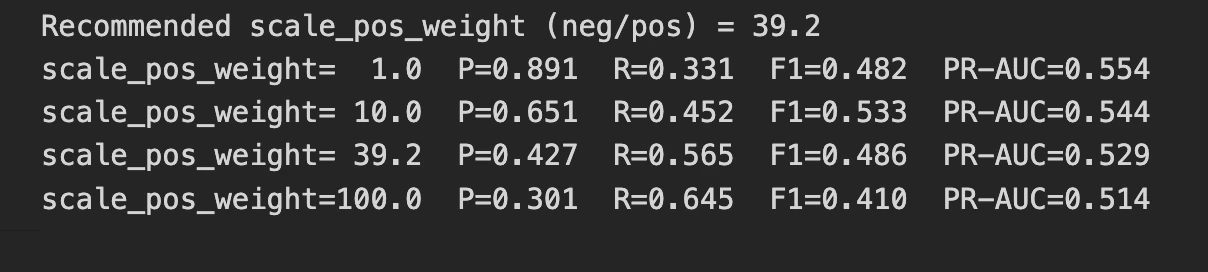
The textbook worth of 39.2 doesn’t give the perfect F1 rating. A tuned worth of 10 wins on F1 with a more healthy precision stability. In the meantime, the threshold-independent PR-AUC barely strikes throughout settings. This confirms that weighting principally shifts the working level, not the rating. Deal with the method as a touch and at all times tune round it.
Code Demo: Isolation Forest on the Minority Class
This demo trains Isolation Forest on majority information solely. We use a dataset the place the minority class is a real outlier group. The mannequin by no means sees minority labels throughout coaching. Watch how properly it recovers the uncommon class anyway.
import numpy as np

from sklearn.model_selection import train_test_split
from sklearn.ensemble import IsolationForest
from sklearn.metrics import (
    average_precision_score,
    precision_score,
    recall_score,
    f1_score,
)


rng = np.random.default_rng(42)

# Majority: a good cluster of "regular" habits. Minority: real outliers.
X_normal = rng.regular(0, 1.0, measurement=(19900, 20))

X_anom = rng.regular(0, 1.0, measurement=(100, 20)) + rng.selection(
    [-6, 6],
    measurement=(100, 20),
) * (rng.random((100, 20)) > 0.6)

Xa = np.vstack([X_normal, X_anom])
ya = np.r_[np.zeros(19900), np.ones(100)].astype(int)

Xtr, Xte, ytr, yte = train_test_split(
    Xa,
    ya,
    test_size=0.25,
    stratify=ya,
    random_state=42,
)

iso = IsolationForest(
    n_estimators=300,
    contamination=0.005,
    random_state=42,
)

iso.match(Xtr[ytr == 0])  # study "regular" solely

scores = -iso.score_samples(Xte)  # increased = extra anomalous
pred = (iso.predict(Xte) == -1).astype(int)  # -1 means anomaly

print(
    f"Isolation Forest  P={precision_score(yte, pred):.3f} "
    f"R={recall_score(yte, pred):.3f} "
    f"F1={f1_score(yte, pred):.3f} "
    f"PR-AUC={average_precision_score(yte, scores):.3f}"
)
Output:

Isolation Forest catches each anomaly with a near-perfect PR-AUC. It achieved this with out ever seeing a single minority label. However this success will depend on the minority being a real outlier. Earlier, on information the place the uncommon class overlapped the bulk, the identical methodology failed utterly.
Code Demo: Weighted Loss in a Neural Internet
This demo trains a small neural community with weighted binary cross-entropy. We evaluate an unweighted loss in opposition to a class-weighted one. The pos_weight argument scales the positive-class contribution to the loss. The PyTorch code beneath exhibits the idiomatic sample you’ll reuse.
import torch
import torch.nn as nn


# X_train, y_train assumed scaled and transformed to tensors
mannequin = nn.Sequential(
    nn.Linear(20, 32),
    nn.ReLU(),
    nn.Linear(32, 1),
)

# pos_weight pushes the loss to care extra in regards to the uncommon optimistic class
pos_weight = torch.tensor([39.0])  # ~ neg / pos ratio

criterion = nn.BCEWithLogitsLoss(pos_weight=pos_weight)
optimizer = torch.optim.Adam(mannequin.parameters(), lr=0.01)

for epoch in vary(200):
    optimizer.zero_grad()

    logits = mannequin(X_train_t).squeeze()
    loss = criterion(logits, y_train_t.float())

    loss.backward()
    optimizer.step()

with torch.no_grad():
    proba = torch.sigmoid(mannequin(X_test_t).squeeze()).numpy()

pred = (proba >= 0.5).astype(int)
The metrics beneath come from coaching an equal one-hidden-layer community with and with out the pos_weight time period, on the identical playground dataset.
Output:

The unweighted community collapses solely and predicts no positives. Its PR-AUC of 0.041 means it can’t rank the minority in any respect. Including pos_weight recovers 74% recall and a much better PR-AUC. Weighted loss is the only, most dependable neural-network repair for imbalance.
Code Demo: PR-AUC vs. ROC-AUC on the Similar Mannequin
This demo computes a full suite of metrics for one mannequin. It contrasts the rosy ROC-AUC with the trustworthy PR-AUC. It additionally experiences MCC, balanced accuracy, and G-Imply for context. The hole between the 2 AUCs is the important thing takeaway.
from sklearn.ensemble import RandomForestClassifier
from sklearn.metrics import (
    roc_auc_score,
    average_precision_score,
    matthews_corrcoef,
    balanced_accuracy_score,
    f1_score,
)
from imblearn.metrics import geometric_mean_score


clf = RandomForestClassifier(
    n_estimators=300,
    random_state=RANDOM_STATE,
    n_jobs=-1,
).match(X_train, y_train)

proba = clf.predict_proba(X_test)[:, 1]
pred = (proba >= 0.5).astype(int)

print(f"ROC-AUC             : {roc_auc_score(y_test, proba):.3f}   <- seems nice")
print(
    f"PR-AUC (avg prec.)  : {average_precision_score(y_test, proba):.3f}   "
    f"<- the trustworthy view"
)
print(f"Base fee (minority): {y_test.imply():.3f}")
print(f"MCC                 : {matthews_corrcoef(y_test, pred):.3f}")
print(f"Balanced accuracy   : {balanced_accuracy_score(y_test, pred):.3f}")
print(f"G-Imply              : {geometric_mean_score(y_test, pred):.3f}")
print(f"F1 (minority)       : {f1_score(y_test, pred):.3f}")
Output:
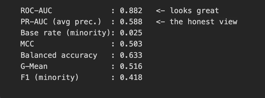
ROC-AUC of 0.882 would persuade most stakeholders the mannequin is superb. PR-AUC of 0.588 reveals there may be nonetheless actual work to do. The 2 metrics describe the identical mannequin but inform totally different tales. All the time report PR-AUC for imbalanced classification, not ROC-AUC alone.
A Sensible Choice Framework
You now have many instruments, so that you want a manner to decide on. A transparent workflow prevents you from defaulting to SMOTE reflexively. The framework beneath strikes from low cost experiments to costly ones. Comply with it, and you’ll not often waste effort on the improper repair.
Step-by-Step Workflow for Tackling a New Imbalanced Drawback
This sequence orders interventions by price and threat. Begin easy, measure actually, and escalate solely when wanted. Every step builds on the proof from the earlier one.
- Construct a robust baseline mannequin and consider it with PR-AUC, not accuracy.
- Tune the choice threshold on a validation set earlier than the rest.
- Add class weights or
scale_pos_weightto make minority errors expensive. - Strive a balanced ensemble resembling Balanced Random Forest.
- Attain for resampling like SMOTE provided that less complicated steps underperform.
- If positives are extraordinarily uncommon, reframe the duty as anomaly detection.
A Choice Desk: Imbalance Ratio → Really useful Method
The fitting approach relies upon partly on how extreme your imbalance is. This desk affords wise beginning factors by imbalance ratio. Deal with them as defaults to check, not inflexible guidelines to obey.
| Imbalance ratio | Minority share | Really useful start line |
|---|---|---|
| As much as 10:1 | Above 10% | Threshold tuning and sophistication weights |
| 10:1 to 100:1 | 1% to 10% | Class weights, balanced ensembles, threshold tuning |
| 100:1 to 1000:1 | 0.1% to 1% | Price-sensitive boosting, focal loss, cautious resampling |
| Above 1000:1 | Beneath 0.1% | Anomaly detection and one-class strategies |
Frequent Pitfalls and Methods to Keep away from Them
Most imbalanced-learning failures come from a couple of repeated errors. Figuring out them upfront saves weeks of confused debugging. Watch fastidiously for every of the next traps.
- Resampling earlier than splitting: This leaks check information into coaching and inflates scores wildly. All the time resample contained in the pipeline.
- Optimizing accuracy: Accuracy rewards ignoring the minority class. Optimize PR-AUC, F1, or a cost-aware metric as a substitute.
- Ignoring calibration: Resampling distorts chances. Recalibrate while you want reliable chance scores for selections.
- Over-synthesizing minority information: Extreme oversampling invents noise and amplifies overlap. Want modest weighting over aggressive synthesis.
Actual-World Instance: Constructing a Fraud Detection Pipeline
Principle issues lower than a working end-to-end comparability. Right here we construct a fraud pipeline and pit three methods in opposition to one another. We evaluate a baseline, a SMOTE pipeline, and a contemporary strategy. The outcomes reveal which technique really earns its place.
The Dataset and Its Imbalance Profile
We reuse our 20,000-row dataset with its 2% minority class. This profile mirrors many actual fraud and rare-event issues. We cut up it into practice, validation, and check units. The validation set exists purely for tuning the choice threshold.
Code Demo: Baseline vs. SMOTE vs. Trendy Method
This pipeline trains three competing fashions on an identical information. The fashionable strategy combines cost-sensitive boosting with threshold tuning. It additionally optimizes PR-AUC throughout coaching fairly than log loss. We then evaluate all three throughout 5 trustworthy metrics.
import numpy as np
from collections import Counter

from sklearn.metrics import (
    precision_score,
    recall_score,
    f1_score,
    average_precision_score,
    matthews_corrcoef,
    precision_recall_curve,
)
from imblearn.over_sampling import SMOTE
from imblearn.pipeline import Pipeline
from xgboost import XGBClassifier


Xtr, Xtmp, ytr, ytmp = train_test_split(
    X,
    y,
    test_size=0.40,
    stratify=y,
    random_state=RANDOM_STATE,
)

Xval, Xte, yval, yte = train_test_split(
    Xtmp,
    ytmp,
    test_size=0.50,
    stratify=ytmp,
    random_state=RANDOM_STATE,
)


def consider(identify, proba, thr=0.5):
    pred = (proba >= thr).astype(int)

    print(
        f"{identify:<28} thr={thr:.3f} "
        f"P={precision_score(yte, pred):.3f} "
        f"R={recall_score(yte, pred):.3f} "
        f"F1={f1_score(yte, pred):.3f} "
        f"PR-AUC={average_precision_score(yte, proba):.3f} "
        f"MCC={matthews_corrcoef(yte, pred):.3f}"
    )


# 1) Baseline
base = XGBClassifier(
    n_estimators=300,
    max_depth=4,
    learning_rate=0.1,
    eval_metric="logloss",
    random_state=RANDOM_STATE,
    n_jobs=-1,
).match(Xtr, ytr)

consider("Baseline XGBoost", base.predict_proba(Xte)[:, 1])


# 2) SMOTE + XGBoost
smote = Pipeline(
    [
        ("smote", SMOTE(random_state=RANDOM_STATE)),
        (
            "clf",
            XGBClassifier(
                n_estimators=300,
                max_depth=4,
                learning_rate=0.1,
                eval_metric="logloss",
                random_state=RANDOM_STATE,
                n_jobs=-1,
            ),
        ),
    ]
).match(Xtr, ytr)

consider("SMOTE + XGBoost", smote.predict_proba(Xte)[:, 1])


# 3) Trendy: cost-sensitive + PR-AUC eval + threshold tuned on validation
fashionable = XGBClassifier(
    n_estimators=300,
    max_depth=4,
    learning_rate=0.1,
    scale_pos_weight=10,
    eval_metric="aucpr",
    random_state=RANDOM_STATE,
    n_jobs=-1,
).match(Xtr, ytr)

val_p = fashionable.predict_proba(Xval)[:, 1]

prec, rec, thr = precision_recall_curve(yval, val_p)
f1s = 2 * prec * rec / (prec + rec + 1e-9)
best_t = thr[np.argmax(f1s[:-1])]

consider(
    "Price-sensitive + tuned thr",
    fashionable.predict_proba(Xte)[:, 1],
    thr=best_t,
)
Output:
Evaluating Outcomes Throughout Metrics
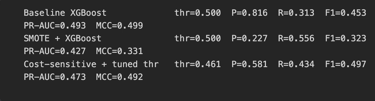
The desk beneath summarizes the three methods aspect by aspect. Learn it throughout the F1, PR-AUC, and MCC columns. The sample challenges the favored religion in computerized SMOTE.
| Mannequin | Precision | Recall | F1 | PR-AUC | MCC |
|---|---|---|---|---|---|
| Baseline XGBoost | 0.816 | 0.313 | 0.453 | 0.493 | 0.499 |
| SMOTE + XGBoost | 0.227 | 0.556 | 0.323 | 0.427 | 0.331 |
| Price-sensitive + tuned threshold | 0.581 | 0.434 | 0.497 | 0.473 | 0.492 |
Classes Discovered
SMOTE truly harm this sturdy gradient booster throughout most metrics. It reduce F1, PR-AUC, and MCC in comparison with the plain baseline. The associated fee-sensitive, threshold-tuned mannequin delivered the perfect F1 and stability. Trendy, model-aware strategies beat reflexive resampling on sensible information.
Verdict: What Ought to You Really Use?
No single approach wins each imbalanced drawback mechanically. The fitting selection will depend on your information, ratio, and prices. Nonetheless, clear patterns emerge from the experiments above. Right here is the best way to match the strategy to the state of affairs.
Conclusion
Imbalanced classification is just not solved by reaching for SMOTE on autopilot. The strongest outcomes got here from low cost, model-aware strikes as a substitute. Threshold tuning, class weights, and balanced ensembles repeatedly beat naive oversampling. In our fraud pipeline, SMOTE truly degraded a succesful gradient booster.
Substitute the “simply use SMOTE” reflex with a principled workflow. Begin with a robust baseline and PR-AUC, then tune the brink. Add price sensitivity, strive balanced ensembles, and think about anomaly detection for rarities. Match the approach to your information, and your skewed-data classifiers will lastly work.
Incessantly Requested Questions
A. When one class seems far much less typically, inflicting fashions to miss uncommon however essential circumstances.
A. Excessive accuracy can conceal a mannequin that predicts solely the bulk class.
A. Begin with PR-AUC, threshold tuning, class weights, and balanced ensembles.

Hiya! I am Vipin, a passionate information science and machine studying fanatic with a robust basis in information evaluation, machine studying algorithms, and programming. I’ve hands-on expertise in constructing fashions, managing messy information, and fixing real-world issues. My aim is to use data-driven insights to create sensible options that drive outcomes. I am desperate to contribute my expertise in a collaborative atmosphere whereas persevering with to study and develop within the fields of Knowledge Science, Machine Studying, and NLP.
Login to proceed studying and revel in expert-curated content material.

