Utilizing Apache Sedona with AWS Glue to course of billions of each day factors from a geospatial dataset

Information technique can use geospatial knowledge to offer organizations with insights for decision-making and operational optimization. By incorporating geospatial knowledge (equivalent to GPS coordinates, factors, polygons and geographic boundaries), companies can uncover patterns, traits, and relationships that may in any other case stay hidden throughout a number of industries, from aviation and transportation to environmental research and concrete planning. Processing and analyzing this geospatial knowledge at scale might be difficult, particularly when coping with billions of each day observations.

On this put up, we discover use Apache Sedona with AWS Glue to course of and analyze huge geospatial datasets.

Introduction to geospatial knowledge

Geospatial knowledge is info that has a geographic element. It describes objects, occasions, or phenomena together with their location on the Earth’s floor. This knowledge consists of coordinates (latitude and longitude), shapes (factors, strains, polygons), and related attributes (such because the identify of a metropolis or the kind of street).

Key kinds of geospatial geometries (and examples of every in parentheses) embody:

• Level – Represents a single coordinate (a climate station).
• MultiPoint – A set of factors (bus stops in a metropolis).
• LineString – A collection of factors related in a line (a river or a flight path).
• MultiLineString – A number of strains (a number of flight routes).
• Polygon – A closed space (the boundary of a metropolis).
• MultiPolygon – A number of polygons (nationwide parks in a rustic).

Geospatial datasets come in several codecs, every designed to retailer and signify several types of geographic info. Widespread codecs for geospatial knowledge are vector codecs (Shapefile, GeoJSON), raster codecs (GeoTIFF, ESRI Grid), GPS codecs (GPX, NMEA), internet codecs (WMS, GeoRSS) amongst others.

Core ideas of Apache Sedona

Apache Sedona is an open-source computing framework for processing large-scale geospatial knowledge. Constructed on prime of Apache Spark, Sedona extends Spark’s capabilities to deal with spatial operations effectively. At its core, Sedona introduces a number of key ideas that allow distributed spatial processing. These embody Spatial Resilient Distributed Datasets (SRDDs), which permit for the distribution of spatial knowledge throughout a cluster, and Spatial SQL, which offers a well-known SQL-like interface for spatial queries. Among the core capabilities of Apache Sedona are:

• Environment friendly spatial knowledge sorts like factors, strains and polygons.
• Spatial operations and features equivalent to ST_Contains (test if level is inside a polygon), ST_Intersects (test if level is inside a polygon), ST_H3CellIDs (geospatial indexing system developed by Uber, return the H3 cell ID(s) that comprise the given level on the specified decision).
• Spatial joins to mix completely different spatial datasets.
• Integration with Spark SQL (geospatial features to run spatial SQL queries).
• Spatial indexing methods, equivalent to quad-trees and R-trees, to optimize question efficiency.

For extra details about the features obtainable in Apache Sedona, go to the official Sedona Features documentation.

Use case

This use case consists of a world air visitors visualization and evaluation platform that processes and shows real-time or historic plane monitoring knowledge on an interactive world map. Utilizing distinctive plane identifiers from the Worldwide Civic Aviation Group (ICAO), the system ingests trajectory information containing info equivalent to geographic place (latitude and longitude), altitude, pace, and flight route, then transforms this uncooked knowledge into two complementary visible layers. The Flight Tracks Layer plots the routes traveled by every plane individually, permitting for the evaluation of particular trajectories and navigation patterns. The Flight Density Layer makes use of hexagonal spatial indexing (H3) to mixture and determine areas of upper air visitors focus worldwide, revealing busy air corridors, aviation hubs, and high-density flight zones.

The dataset used for this use case is historic flight tracker knowledge from ADSB.lol. ADSB.lol offers unfiltered flight tracker with a give attention to open knowledge. Information can be freely obtainable by way of the API. The information comprises a file per plane, a JSON gzip file containing the information for that plane for the day.

This can be a JSON hint file format pattern:

{
    icao: "0123ac", // hex id of the plane
    timestamp: 1609275898.495, // unix timestamp in seconds since epoch (1970)
    hint: [
        [ seconds after timestamp,
            lat,
            lon,
            altitude in ft or "ground" or null,
            ground speed in knots or null,
            track in degrees or null, (if altitude == "ground", this will be true heading instead of track)
            flags as a bitfield: (use bitwise and to extract data)
                (flags & 1 > 0): position is stale (no position received for 20 seconds before this one)
                (flags & 2 > 0): start of a new leg (tries to detect a separation point between landing and takeoff that separates flights)
                (flags & 4 > 0): vertical rate is geometric and not barometric
                (flags & 8 > 0): altitude is geometric and not barometric
             ,
            vertical rate in fpm or null,
            aircraft object with extra details or null,
            type / source of this position or null,
            geometric altitude or null,
            geometric vertical rate or null,
            indicated airspeed or null,
            roll angle or null
        ],
    ]
}

For this use case, it is a simplified schema of the dataset after processing:

• icao - Distinctive plane identifier
• timestamp - Epoch timestamp of the statement (transformed to readable format)
• hint.lat / hint.lon - Latitude and longitude of the plane
• hint.altitude - Plane altitude
• hint.ground_speed - Floor pace
• geometry - Geospatial geometry of the statement level (Level)

Answer overview

This resolution permits plane monitoring and evaluation. The information might be visualized on maps and used for aviation administration and security purposes. The method begins with knowledge acquisition, extracting the compressed JSON recordsdata from TAR archives, then transforms this uncooked knowledge into geospatial objects, aggregating them into H3 cells for environment friendly evaluation. The processed knowledge schema consists of ICAO plane identifiers, timestamps, latitude/longitude coordinates, and derived fields equivalent to H3 cell identifiers and level counts per cell. This construction permits detailed monitoring of particular person flights and mixture evaluation of visitors patterns. For visualization, you may generate density maps utilizing the H3 grid system and create visible representations of particular person flight tracks. The structure knowledge movement is as follows:

• Information ingestion – Plane statement knowledge saved as JSON compressed recordsdata in Amazon Easy Storage Service (Amazon S3).
• Information processing – AWS Glue jobs utilizing Apache Sedona for geospatial processing.
• Information visualization – Spark SQL with Sedona’s spatial features to extract insights and export knowledge to visualise the knowledge in a map on Kepler.gl.

The next determine illustrates this resolution.

Conditions

You will want the next for this resolution:

• An AWS Account and a person with AWS Console entry.
• Entry to a Linux terminal and the AWS Command Line Interface (AWS CLI).
• An IAM position for AWS Glue with checklist, learn, and write permissions for Amazon S3 buckets.
• An Amazon S3 Bucket for flight recordsdata. For this instance, identify the bucket blog-sedona-nessie--, utilizing your account quantity and area.
• An Amazon S3 bucket for artifacts and Sedona libraries. For this instance, identify the bucket blog-sedona-artifacts--, utilizing your account quantity and area.
• Obtain a day of historic knowledge from ADSB.lol. In our examples, we used v2025.05.29-planes-readsb-prod-0tmp.tar.aa and v2025.05.29-planes-readsb-prod-0tmp.tar.ab.
• Obtain the Apache Sedona libraries. The instance was created utilizing sedona-spark-shaded-3.5_2.12-1.7.1.jar and geotools-wrapper-1.7.1-28.5.jar.
• Obtain the AWS Glue script from AWS Pattern to course of the geospatial knowledge.
• Evaluate the AWS Glue safety finest practices, particularly IAM least-privilege, encryption for delicate knowledge at relaxation and in transit, and configuring VPC Endpoints to forestall knowledge from routing via the general public web.

Answer walkthrough

To any extent further, executing the subsequent steps will incur prices on AWS. This step-by-step walkthrough demonstrates an method to processing and analyzing large-scale geospatial flight knowledge utilizing Apache Sedona and Uber’s H3 spatial indexing system, utilizing AWS Glue for distributed processing and Apache Sedona for environment friendly geospatial computations. It explains ingest uncooked flight knowledge, remodel it utilizing Sedona’s geospatial features, and index it with H3 for optimized spatial queries. Lastly, it additionally demonstrates visualize the information utilizing Kepler.gl. For knowledge processing, it’s attainable to make use of each Glue scripts and Glue notebooks. On this put up, we’ll focus solely on Glue scripts.

Add the Apache Sedona libraries to Amazon S3

1. Open your OS terminal command line.
2. Create a folder to obtain the Sedona libraries and identify it jar.

   
   	# Create a listing for the Sedona libraries (JARs recordsdata)
   	mkdir jar
   	# Go to the folder JARs folder
   	cd jar
   	

3. Obtain the Apache Sedona libraries.

   
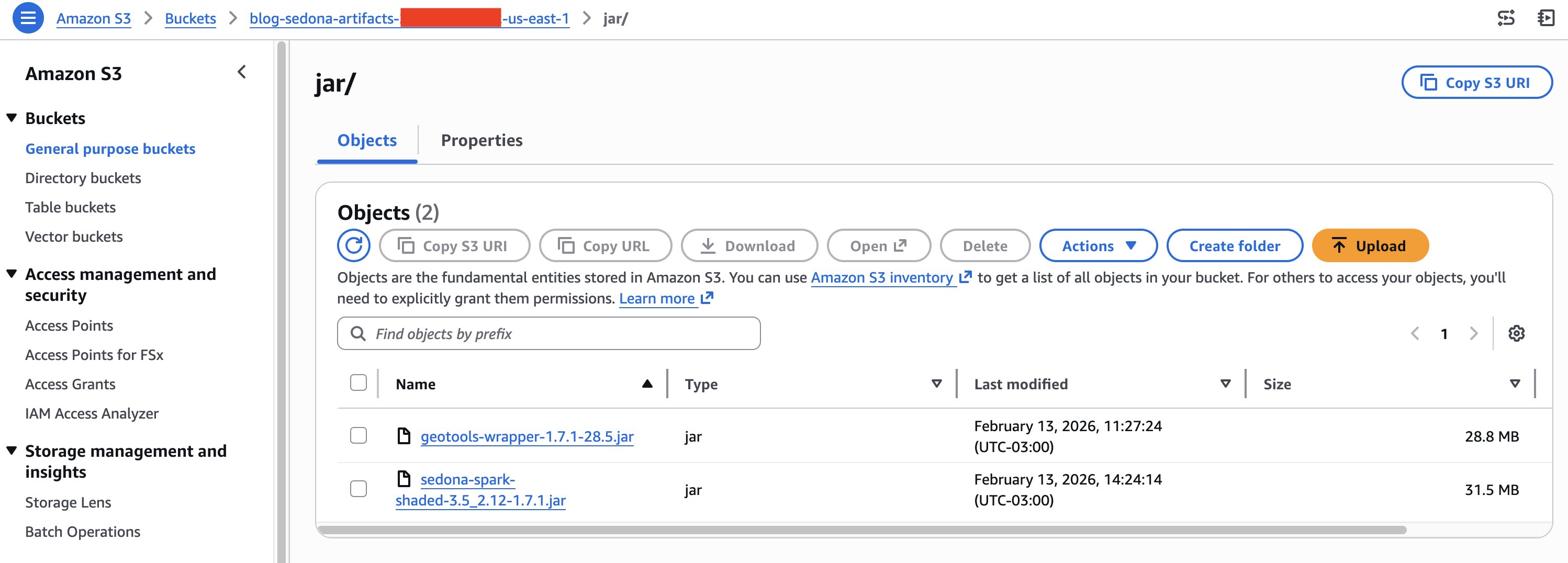
   	# Obtain required Sedona libraries (JARs recordsdata)
   	wget https://repo1.maven.org/maven2/org/apache/sedona/sedona-spark-shaded-3.5_2.12/1.7.1/sedona-spark-shaded-3.5_2.12-1.7.1.jar
   	wget https://repo1.maven.org/maven2/org/datasyslab/geotools-wrapper/1.7.1-28.5/geotools-wrapper-1.7.1-28.5.jar
   	

4. Add the Sedona libraries (JARs recordsdata) to Amazon S3. On this instance, we use the S3 path s3://aws-blog-post-sedona-artifacts/jar/.

   
   	# Add the JARs recordsdata to Amazon S3 bucket
   	aws s3 cp . s3://blog-sedona-artifacts--/jar/ --recursive
   	

5. Your Amazon S3 folder ought to now look much like the next picture:

Obtain and add the geospatial knowledge to Amazon S3

1. Open your OS terminal command line.
2. Create a folder to obtain the flight recordsdata and identify it adsb_dataset.

   		# Create a listing for obtain the geospatial flight recordsdata
   		mkdir adsb_dataset
   		# Go to the folder for geospatial flight recordsdata
   		cd adsb_dataset
   	

3. Obtain the flight recordsdata knowledge from adsblol GitHub repository.

   	# Obtain the geospatial flight recordsdata within the folder created
   	wget https://github.com/adsblol/globe_history_2025/releases/obtain/v2025.05.29-planes-readsb-prod-0tmp/v2025.05.29-planes-readsb-prod-0tmp.tar.aa
   	wget https://github.com/adsblol/globe_history_2025/releases/obtain/v2025.05.29-planes-readsb-prod-0tmp/v2025.05.29-planes-readsb-prod-0tmp.tar.ab
   	

4. Extract the flight recordsdata.

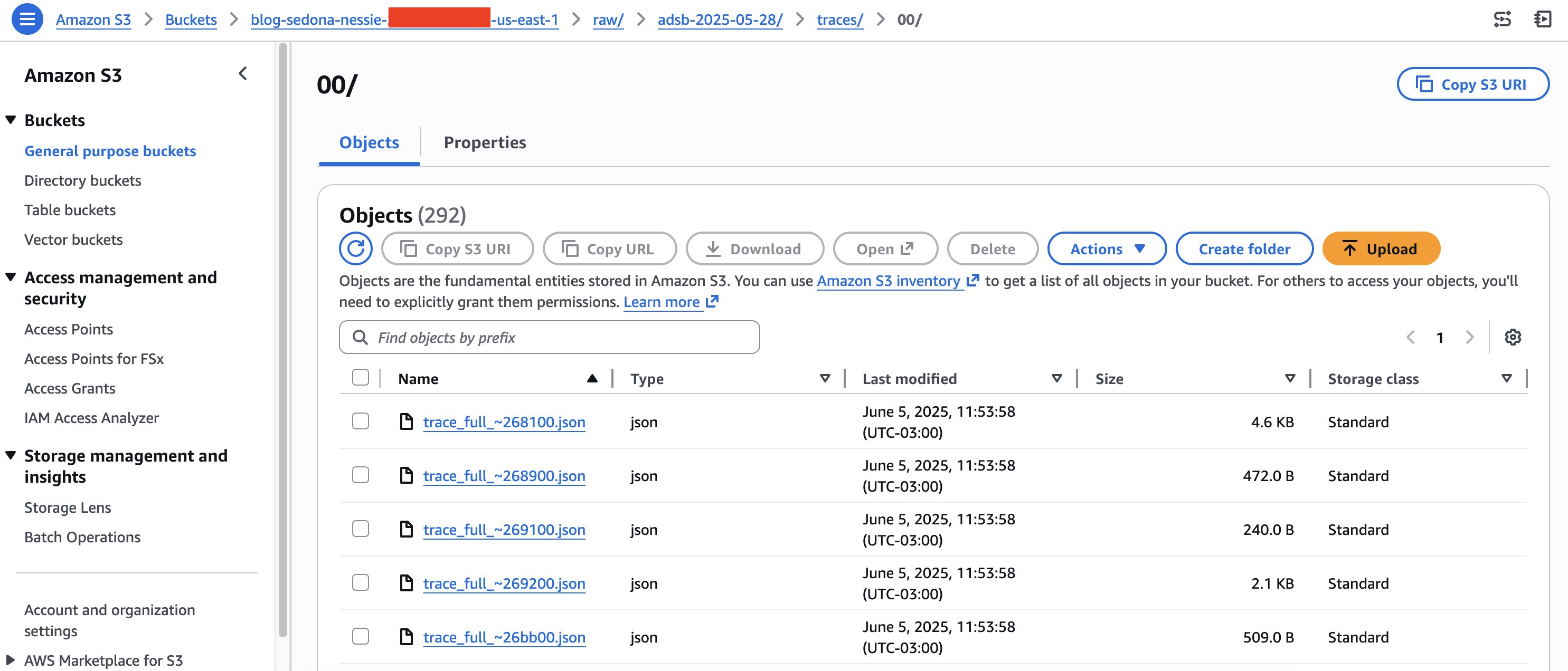
   	# Mix the 2 the tar recordsdata collectively
   	cat v2025.05.29* >> mixed.tar
   	# Extract the json flight recordsdata from the tar file
   	tar xf mixed.tar
   	

5. Copy the flight recordsdata to Amazon S3. On this case, we’re utilizing the S3 folder: s3://blog-sedona-nessie--/uncooked/adsb-2025-05-28/traces/.

   	# Copy the json flight recordsdata to Amazon S3
   	aws s3 cp ./traces/ s3://blog-sedona-nessie--/uncooked/adsb-2025-05-28/traces/ --recursive
   	

6. Your Amazon S3 folder ought to now look much like the next picture.

Create an AWS Glue job and arrange the job

Now, we’re able to outline the AWS Glue job utilizing Apache Sedona to learn the geospatial knowledge recordsdata. To create a Glue job:

1. Open the AWS Glue console.
2. On the Notebooks web page, select Script editor.

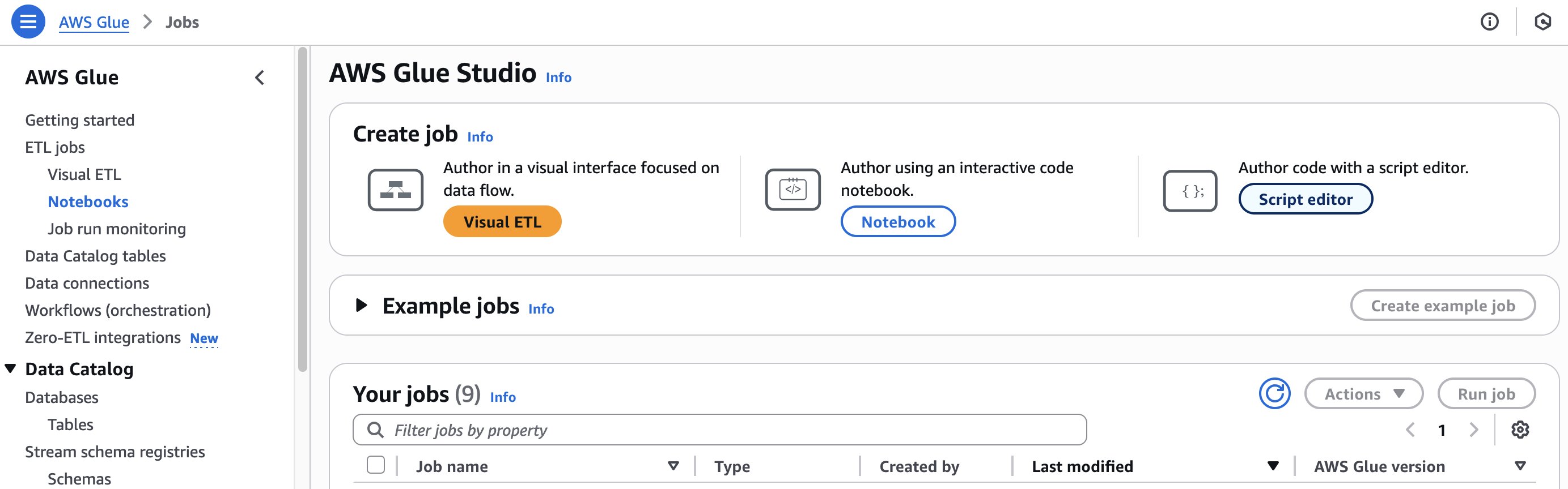
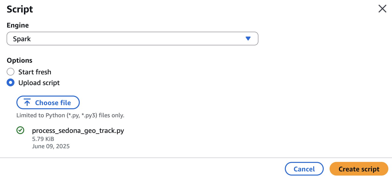
3. On the Script display, for the engine, select Spark, then choose the choice Add script.
4. Select Select file. Discover the process_sedona_geo_track.py file, then select Create script.

5. Rename the job from Untitled to process_sedona_geo_track.
6. Select Save.
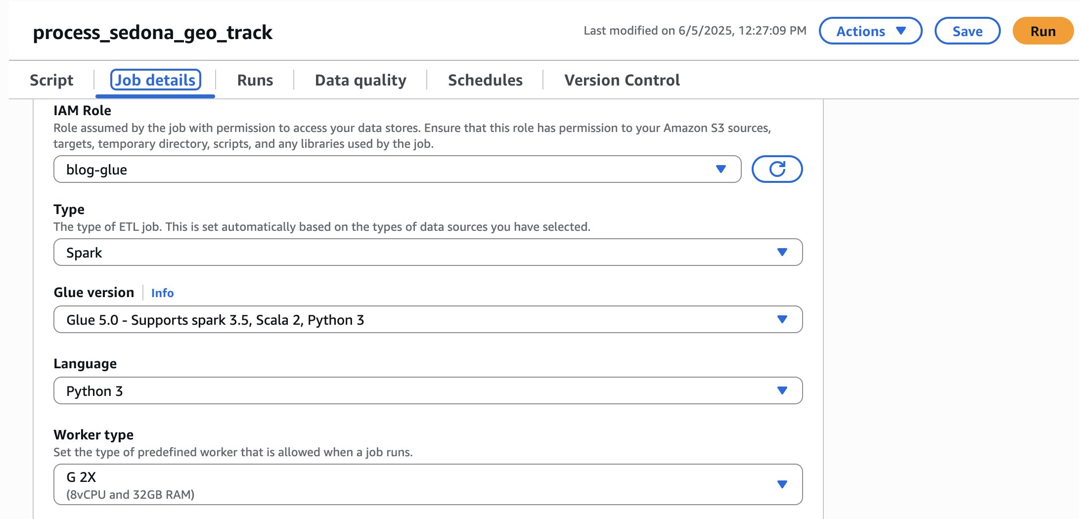
7. Now, let’s arrange the AWS Glue job. Select Job Particulars.
8. Select the IAM Function created for use with Glue. For this instance, we use blog-glue.
9. Set the Glue model to Glue 5.0 and the Employee sort as wanted. For this instance, G.1X is enough, however we use G.2X to hurry up processing.

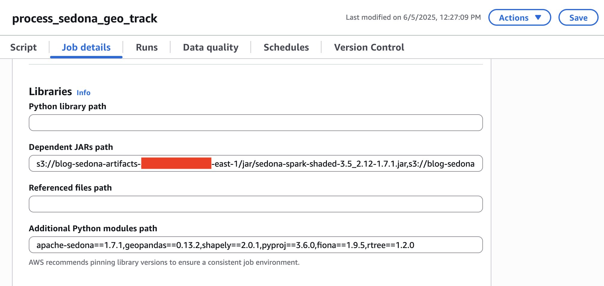
10. Now, let’s import the libraries for Apache Sedona.
11. Within the Dependent JARs path, sort the trail of the JAR recordsdata for Apache Sedona that you simply uploaded within the previous steps. For this instance, we used s3://blog-sedona-artifacts--/jar/sedona-spark-shaded-3.5_2.12-1.7.1.jar,s3://blog-sedona-artifacts--/jar/geotools-wrapper-1.7.1-28.5.jar
12. In Extra Python modules path, enter the modules for Apache Sedona: apache-sedona==1.7.1,geopandas==0.13.2,shapely==2.0.1,pyproj==3.6.0,fiona==1.9.5,rtree==1.2.0

13. Within the Job parameters part, within the Key area, sort —BUCKET_NAME. For its Worth, enter your bucket identify. On this instance, ours is blog-sedona-nessie--.

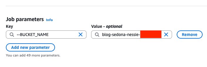
14. Select Save.

Processing the geospatial flights knowledge

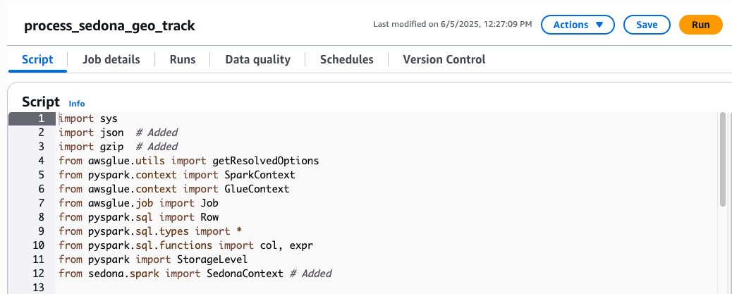
Earlier than we run the job, let’s perceive how the code works. First, import the Apache Sedona libraries:

import json 
import gzip 
from sedona.spark import SedonaContext

Subsequent, initialize the Sedona context utilizing an current Spark session:

sedona = SedonaContext.create(spark)

After that, create a operate for dealing with compressed JSON knowledge:

def parse_gzip_json(byte_content):
        attempt:
            decompressed = gzip.decompress(byte_content)
            return json.hundreds(decompressed.decode('utf-8'))
        besides Exception as e:
            print(f"Error throughout gzip parse: {str(e)}")
            return None

Add a operate to remodel uncooked monitoring knowledge right into a structured format appropriate for a legitimate coordinates course of:

def flatten_records(json_obj):
    information = []
    if "hint" in json_obj and isinstance(json_obj["trace"], checklist):
        for level in json_obj["trace"]:
            if len(level) >= 3:
                lat, lon = float(level[1]), float(level[2])
                if -90 <= lat <= 90 and -180 <= lon <= 180:
                    information.append(Row(
                        icao=json_obj.get("icao", None),
                        timestamp=json_obj.get("timestamp", None),
                        lat=lat,
                        lon=lon
                    ))
    return information

The flat_rdd variable applies these features to the structured knowledge from the unique gzipped JSON. Every factor on this RDD is a Row object representing a single knowledge level from an plane’s hint, with fields for ICAO, timestamp, latitude, and longitude.

flat_rdd = raw_rdd.map(lambda x: parse_gzip_json(x[1])).filter(lambda x: x shouldn't be None).flatMap(flatten_records)

The ADSB hint recordsdata comprise a deeply nested JSON construction the place the hint area holds an array of mixed-type arrays, compressed in Gzip format. For this particular case, creating a UDF represented probably the most sensible and environment friendly options. Since Gzip is a non-splittable format, Spark is unable to parallelize processing, constraining each strategies to a single employee per file and processing the information a number of occasions throughout JVM decompression, full JSON parsing, and subsequent re-parsing operations. The UDF bypasses all of this by studying uncooked bytes and doing all the pieces in a single Python move: decompress → parse → extract → validate, returning solely the small set of wanted fields on to Spark.

The Spark SQL question processes geographic hint knowledge utilizing the H3 hexagonal grid system, changing level knowledge right into a regularized hexagonal grid that may assist determine areas of excessive level density. A decision of 5 was adopted, producing hexagons of roughly 253 km² (roughly the identical measurement as the town of Edinburgh, Scotland, which is roughly 264 km²), for its capability to successfully seize route density patterns on the metropolis and metropolitan stage.

h3_traces_df = spark.sql("""
WITH base_h3 AS (
    SELECT
        ST_H3CellIDs(geometry, 5, false)[0] AS h3_index,
        lat,
        lon
    FROM traces
)
SELECT
    COUNT(*) AS num, -- Depend factors in every H3 cell
    h3_index,
    AVG(lon) AS center_lon,
    AVG(lat) AS center_lat
FROM base_h3
GROUP BY h3_index
""")

Lastly, this code prepares the datasets for visualization functions. The primary dataset relies on the plane distinctive identifier. The whole dataset for a single day can comprise greater than 80 million knowledge factors. A random sampling price of 0.1% was utilized, which proves enough as an instance route density patterns with out overwhelming the Kepler.gl browser renderer. The second dataset aggregates hint factors into hexagonal spatial cells (outcome from the question above).

points_viz_sampled = df_points.choose(
    col("icao"), # Plane distinctive identifier (24-bit handle)
    col("timestamp").solid("double").alias("timestamp"),
    col("lat").solid("double").alias("lat"),
    col("lon").solid("double").alias("lon")
).pattern(False, 0.001)

h3_viz_csv = h3_traces_df.choose(
    col("num").alias("point_count"),
    col("h3_index").solid("string").alias("h3_index"),
    col("center_lon"),
    col("center_lat")
)

Now that we perceive the code, let’s run it.

1. Open the AWS Glue console.
2. On the ETL jobs >> Notebooks web page, select the job identify process_sedona_geo_track.
3. Select Run.

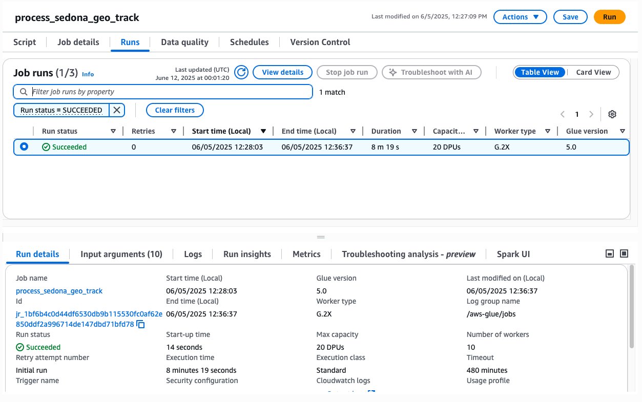
4. Now, it’s attainable to watch the job by selecting the Runs tab.
5. It could take a couple of minutes to run your entire job. It took practically 8 minutes to course of roughly 2.50 GB (67,540 compressed recordsdata) with 20 DPUs. After the job is processed, you must see your job with the standing Succeeded.

Now your knowledge ought to be saved for a preview visualization demo in a folder named s3://blog-sedona-nessie--/visualization/.

Efficiency insights

The workload characterization of this job reveals a CPU-intensive profile, primarily due to the processing of small binary recordsdata with GZIP compression and subsequent JSON parsing. Given the inherent nature of this pipeline, which incorporates Python UDF serialization and partial single-partition write levels, linear scaling doesn’t yield proportional efficiency good points. The next desk presents an evaluation of AWS Glue configurations, evaluating the trade-off between computational capability, execution period, and related prices:

*Estimated Price = DPUs x Period (hours) x $0.44 per DPU-hour (us-east-1)

Visualizing and analyzing geospatial knowledge with Kepler.gl

Kepler.gl is an open-source geospatial evaluation instrument developed by Uber with code obtainable at Github. Kepler.gl is designed for large-scale knowledge exploration and visualization, providing a number of map layers, together with level, arc, heatmap, and 3D hexagon. It helps numerous file codecs like CSV, GeoJSON, and KML. On this use case, we’ll use Kepler.gl to current interactive visualizations that illustrate flight patterns, routes, and densities throughout international airspace.

Downloading the geospatial recordsdata

Earlier than we are able to view the graph, we might want to obtain the flight recordsdata to our native machine, unzip them, and rename them (to make it simpler to determine the recordsdata).

1. Open your OS terminal command line.
2. Create the folders to obtain the information processed within the steps earlier than. On this case, we create kepler and kepler_csv.

   	#create kepler folders: first folder is to obtain the recordsdata,
   	#second folder is to prepare the recordsdata to make use of within the subsequent step
   	mkdir kepler
   	mkdir kepler_csv
   	

3. Substitute the bracketed variables together with your account and listing info, then obtain all of the CSV recordsdata.

   	#copy the recordsdata from Amazon S3 to native machine
   	aws s3 cp s3://blog-sedona-nessie--/visualization/ //kepler --recursive
   	

4. Extract the recordsdata, rename them, and transfer them to a different folder.

   	# Extract the recordsdata processed by Spark and Sedona
   	gzip -d ./kepler/kepler_h3_density/*.gz
   	gzip -d ./kepler/kepler_track_points_sample/*.gz
   	
   	# Rename the Spark output recordsdata to extra readable names
   	cd ./kepler/kepler_h3_density/
   	ls
   	mv part-00000-*.csv kepler_h3_density.csv
   	cd ..
   	
   	cd ./kepler/kepler_track_points_sample/
   	ls
   	mv part-00000-*.csv kepler_track_points_sample.csv
   	cd ..
   	
   	# Make sure the output folder exists
   	mkdir -p ../kepler_csv
   	
   	# Copy the renamed CSV recordsdata to the folder that will probably be used as enter in kepler.gl
   	cp ./kepler/kepler_h3_density/*.csv ../kepler_csv
   	cp ./kepler/kepler_track_points_sample/*.csv ../kepler_csv
   	

5. Your kepler_csv folder ought to look much like the return of the command under.

   	#checklist the recordsdata within the kepler_csv listing
   	ls -l
   	whole 11684
   	-rw-rw-r-- 1 ec2-user ec2-user 8630110 Jun 12 14:47 kepler_h3_density.csv
   	-rw-rw-r-- 1 ec2-user ec2-user 3331763 Jun 12 14:47 kepler_track_points_sample.csv
   	

Visualizing the information in a graph

Now that you’ve got saved the information to your native machine, you may analyze the flight knowledge via interactive map graphics. To import the information into the Kepler.gl internet visualization instrument:

1. Open the Kepler.gl Demo internet software.
2. Load knowledge into Kepler.gl:
   1. Select Add Information within the left panel.
   2. Drag and drop each CSV recordsdata (flight_points and h3_density) into the add space.
   3. Verify that each datasets are loaded efficiently.
3. Delete all layers.
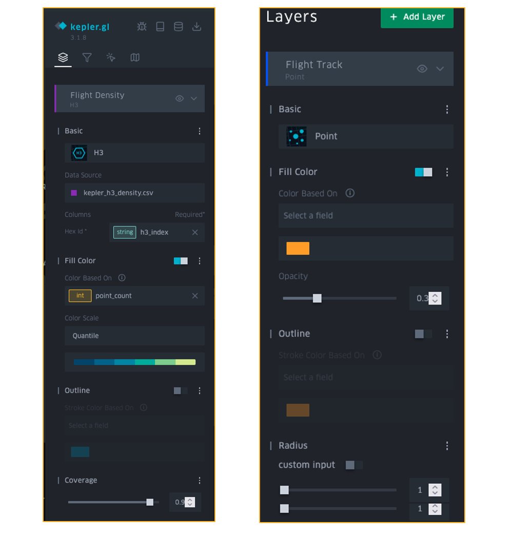
4. Create the Flight Density Layer:
   1. Select Add Layer within the left panel.
   2. In Fundamental, select H3 because the layer sort, then add the next configuration:
      1. Layer Title: Flight Density
      2. Information Supply: kepler_h3_density.csv
      3. Hex ID: h3_index
   3. Within the Fill Shade part:
      1. Shade: point_count
      2. Shade Scale: Quantile.
      3. Shade Vary: Select a blue/inexperienced gradient.
   4. Set Opacity to 0.7.
   5. Within the Protection part, set it to 0.9.
5. Create the Flight Tracks Layer:
   1. Select Add Layer within the left panel.
   2. In Fundamental, select Level because the layer sort, then add the next configuration:
      1. Layer Title: Flight Tracks
      2. Information Supply: kepler_track_points_sample.csv
      3. Columns:
         1. Latitude: lat
         2. Longitude: lon
   3. Within the Fill Shade part:
      1. Strong Shade: Orange
      2. Opacity: 0.3
   4. Set the Level’s Radius to 1
6. The layers ought to look much like the next determine.

7. The graph visualization ought to now present flight density via color-coded hexagons, with particular person flight tracks seen as orange factors:

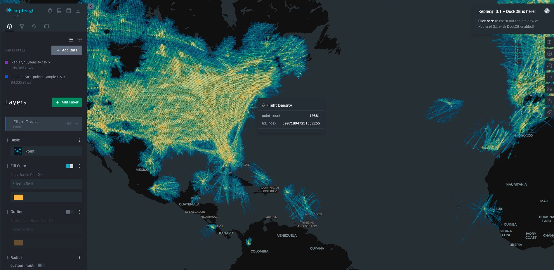
There you go! Now that you’ve got data about geospatial knowledge and have created your first use case, take the chance to do some evaluation and study some attention-grabbing details about flight patterns.

It’s attainable to experiment with different attention-grabbing kinds of evaluation in Kepler.gl, equivalent to Time Playback.

Clear up

To wash up your assets, full the next duties:

1. Delete the AWS Glue job process_sedona_geo_track.
2. Delete content material from the Amazon S3 buckets: blog-sedona-artifacts-- and blog-sedona-nessie--.

Conclusion

On this put up, we confirmed how processing geospatial knowledge can current important challenges as a result of its complicated nature (from large knowledge to knowledge construction format). For this use case of flight trackers, it entails huge quantities of knowledge throughout a number of dimensions equivalent to time, location, altitude, and flight paths, nevertheless, the mixture of Spark’s distributed computing capabilities and Sedona’s optimized geospatial features helps overcome these challenges. The spatial partitioning and indexing options of Sedona, coupled with Spark’s framework, allow us to carry out complicated spatial joins and proximity analyses effectively, simplifying the general knowledge processing workflow.

The serverless nature of AWS Glue eliminates the necessity for managing infrastructure whereas mechanically scaling assets based mostly on workload calls for, making it a really perfect platform for processing rising volumes of flight knowledge. As the amount of flight knowledge grows or as processing necessities fluctuate, with AWS Glue, you may rapidly regulate assets to fulfill demand, guaranteeing optimum efficiency with out the necessity for cluster administration.

By changing the processed outcomes into CSV format and visualizing them in Kepler.gl, it’s attainable to create interactive visualizations that reveal patterns in flight paths, and you may effectively analyze air visitors patterns, routes, and different insights. This end-to-end resolution demonstrates how a contemporary knowledge technique in AWS with the assist of open-source instruments can remodel uncooked geospatial knowledge into actionable insights.

In regards to the authors