

On this article, you’ll learn to construct a deterministic, multi-tier retrieval-augmented technology system utilizing data graphs and vector databases.
Matters we are going to cowl embrace:
- Designing a three-tier retrieval hierarchy for factual accuracy.
- Implementing a light-weight data graph.
- Utilizing prompt-enforced guidelines to resolve retrieval conflicts deterministically.

Past Vector Search: Constructing a Deterministic 3-Tiered Graph-RAG System
Picture by Editor
Introduction: The Limits of Vector RAG
Vector databases have lengthy since turn into the cornerstone of contemporary retrieval augmented technology (RAG) pipelines, excelling at retrieving long-form textual content primarily based on semantic similarity. Nevertheless, vector databases are notoriously “lossy” relating to atomic info, numbers, and strict entity relationships. An ordinary vector RAG system would possibly simply confuse which workforce a basketball participant at present performs for, for instance, just because a number of groups seem close to the participant’s title in latent house. To unravel this, we want a multi-index, federated structure.
On this tutorial, we are going to introduce such an structure, utilizing a quad retailer backend to implement a data graph for atomic info, backed by a vector database for long-tail, fuzzy context.
However right here is the twist: as an alternative of counting on advanced algorithmic routing to choose the suitable database, we are going to question all databases, dump the outcomes into the context window, and use prompt-enforced fusion guidelines to drive the language mannequin (LM) to deterministically resolve conflicts. The objective is to aim to eradicate relationship hallucinations and construct absolute deterministic predictability the place it issues most: atomic info.
Structure Overview: The three-Tiered Hierarchy
Our pipeline enforces strict knowledge hierarchy utilizing three retrieval tiers:
- Precedence 1 (absolute graph info): A easy Python QuadStore data graph containing verified, immutable floor truths structured in Topic-Predicate-Object plus Context (SPOC) format.
- Precedence 2 (statistical graph knowledge): A secondary QuadStore containing aggregated statistics or historic knowledge. This tier is topic to Precedence 1 override in case of conflicts (e.g. a Precedence 1 present workforce reality overrides a Precedence 2 historic workforce statistic).
- Precedence 3 (vector paperwork): An ordinary dense vector DB (ChromaDB) for common textual content paperwork, solely used as a fallback if the data graphs lack the reply.
Atmosphere & Stipulations Setup
To comply with alongside, you will want an surroundings operating Python, a neighborhood LM infrastructure and served mannequin (we use Ollama with llama3.2), and the next core libraries:
- chromadb: For the vector database tier
- spaCy: For named entity recognition (NER) to question the graphs
- requests: To work together with our native LM inference endpoint
- QuadStore: For the data graph tier (see QuadStore repository)
|
# Set up required libraries pip set up chromadb spacy requests
# Obtain the spaCy English mannequin python –m spacy obtain en_core_web_sm |
You may manually obtain the easy Python QuadStore implementation from the QuadStore repository and place it someplace in your native file system to import as a module.
⚠️ Observe: The complete challenge code implementation is obtainable in this GitHub repository.
With these conditions dealt with, let’s dive into the implementation.
Step 1: Constructing a Light-weight QuadStore (The Graph)
To implement Precedence 1 and Precedence 2 knowledge, we use a customized light-weight in-memory data graph referred to as a quad retailer. This information graph shifts away from semantic embeddings towards a strict node-edge-node schema identified internally as a SPOC (Topic-Predicate-Object plus Context).
This QuadStore module operates as a highly-indexed storage engine. Below the hood, it maps all strings into integer IDs to stop reminiscence bloat, whereas protecting a four-way dictionary index (spoc, pocs, ocsp, cspo) to allow constant-time lookups throughout any dimension. Whereas we gained’t dive into the small print of the inner construction of the engine right here, using the API in our RAG script is extremely easy.
Why use this straightforward implementation as an alternative of a extra sturdy graph database like Neo4j or ArangoDB? Simplicity and velocity. This implementation is extremely light-weight and quick, whereas having the extra good thing about being simple to grasp. That is all that’s wanted for this particular use case with out having to study a fancy graph database API.
There are actually solely a few QuadStore strategies it’s essential to perceive:
add(topic, predicate, object, context): Provides a brand new reality to the data graphquestion(topic, predicate, object, context): Queries the data graph for info that match the given topic, predicate, object, and context
Let’s initialize the QuadStore appearing as our Precedence 1 absolute reality mannequin:
|
from quadstore import QuadStore
# Initialize info quadstore facts_qs = QuadStore()
# Natively add info (Topic, Predicate, Object, Context) facts_qs.add(“LeBron James”, “likes”, “coconut milk”, “NBA_trivia”) facts_qs.add(“LeBron James”, “played_for”, “Ottawa Beavers”, “NBA_2023_regular_season”) facts_qs.add(“Ottawa Beavers”, “obtained”, “LeBron James”, “2020_expansion_draft”) facts_qs.add(“Ottawa Beavers”, “based_in”, “downtown Ottawa”, “NBA_trivia”) facts_qs.add(“Kevin Durant”, “is”, “an individual”, “NBA_trivia”) facts_qs.add(“Ottawa Beavers”, “had”, “worst first yr of any growth workforce in NBA historical past”, “NBA_trivia”) facts_qs.add(“LeBron James”, “average_mpg”, “12.0”, “NBA_2023_regular_season”) |
As a result of it makes use of the an identical underlying class, you possibly can populate Precedence 2 (which handles broader statistics and numbers) identically or by studying from a previously-prepared JSONLines file. This file was created by operating a easy script that learn the 2023 NBA common season stats from a CSV file that was freely-acquired from a basketball stats web site (although I can not recall which one, as I’ve had the info for a number of years at this level), and transformed every row right into a quad. You may obtain the pre-processed NBA 2023 stats file in JSONL format from the challenge repository.
Step 2: Integrating the Vector Database
Subsequent, we set up our Precedence 3 layer: the usual dense vector DB. We use ChromaDB to retailer textual content chunks that our inflexible data graphs might need missed.
Right here is how we initialize a persistent assortment and ingest uncooked textual content into it:
|
1 2 3 4 5 6 7 8 9 10 11 12 13 14 15 16 17 18 19 20 21 22 23 24 25 26 27 28 29 |
import chromadb from chromadb.config import Settings
# Initialize vector embeddings chroma_client = chromadb.PersistentClient( path=“./chroma_db”, settings=Settings(anonymized_telemetry=False) ) assortment = chroma_client.get_or_create_collection(title=“basketball”)
# Our fallback unstructured textual content chunks doc1 = ( “LeBron injured for the rest of NBA 2023 seasonn” “LeBron James suffered an ankle damage early within the season, which led to him enjoying far “ “fewer minutes per recreation than he has not too long ago averaged in different seasons. The damage bought a lot “ “worse at the moment, and he’s out for the remainder of the season.” ) doc2 = ( “Ottawa Beaversn” “The Ottawa Beavers star participant LeBron James is out for the remainder of the 2023 NBA season, “ “after his ankle damage has worsened. The groups’ abysmal common season document might find yourself “ “being the worst of any workforce ever, with solely 6 wins as of now, with solely 4 gmaes left in “ “the common season.” )
assortment.upsert( paperwork=[doc1, doc2], ids=[“doc1”, “doc2”] ) |
Step 3: Entity Extraction & International Retrieval
How can we question deterministic graphs and semantic vectors concurrently? We bridge the hole utilizing NER by way of spaCy.
First, we extract entities in fixed time from the person’s immediate (e.g. “LeBron James” and “Ottawa Beavers”). Then, we fireplace off parallel queries to each QuadStores utilizing the entities as strict lookups, whereas querying ChromaDB utilizing string similarity over the immediate content material.
|
1 2 3 4 5 6 7 8 9 10 11 12 13 14 15 16 17 18 19 20 21 22 23 |
import spacy
# Load our NLP mannequin nlp = spacy.load(“en_core_web_sm”)
def extract_entities(textual content): “”“ Extract entities from the given textual content utilizing spaCy. Utilizing set eliminates duplicates. ““” doc = nlp(textual content) return checklist(set([ent.text for ent in doc.ents]))
def get_facts(qs, entities): “”“ Retrieve info for an inventory of entities from the QuadStore (querying topics and objects). ““” info = [] for entity in entities: subject_facts = qs.question(topic=entity) object_facts = qs.question(object=entity) info.prolong(subject_facts + object_facts) # Deduplicate info and return return checklist(set(tuple(reality) for reality in info)) |
We now have all of the retrieved context separated into three distinct streams (facts_p1, facts_p2, and vec_info).
Step 4: Immediate-Enforced Battle Decision
Typically, advanced algorithmic battle decision (like Reciprocal Rank Fusion) fails when resolving granular info in opposition to broad textual content. Right here we take a radically easier method that, as a sensible matter, additionally appears to work properly: we embed the “adjudicator” ruleset immediately into the system immediate.
By assembling the data into explicitly labeled [PRIORITY 1], [PRIORITY 2], and [PRIORITY 3] blocks, we instruct the language mannequin to comply with specific logic when outputting its response.
Right here is the system immediate in its entirety:
|
1 2 3 4 5 6 7 8 9 10 11 12 13 14 15 16 17 18 19 20 21 22 23 24 25 26 27 28 29 30 31 32 33 34 35 36 |
def create_system_prompt(info, stats, data): # Format graph info into easy declarative sentences for language mannequin comprehension formatted_facts = “n”.be a part of([f“In {q[3]}, {q[0]} {str(q[1]).substitute(‘_’, ‘ ‘)} {q[2]}.” if len(q) >= 4 else str(q) for q in info]) formatted_stats = “n”.be a part of([f“In {q[3]}, {q[0]} {str(q[1]).substitute(‘_’, ‘ ‘)} {q[2]}.” if len(q) >= 4 else str(q) for q in stats])
# Convert retrieved data dict to a string of textual content paperwork retrieved_context = “” if data and ‘paperwork’ in data and data[‘documents’]: retrieved_context = ” “.be a part of(data[‘documents’][0])
return f“”“You’re a strict data-retrieval AI. Your ONLY data comes from the textual content offered beneath. It’s essential to fully ignore your inside coaching weights.
PRIORITY RULES (strict): 1. If Precedence 1 (Information) accommodates a direct reply, use ONLY that reply. Don’t complement, qualify, or cross-reference with Precedence 2 or Vector knowledge. 2. Precedence 2 knowledge makes use of abbreviations and should seem to contradict P1 — it’s supplementary background solely. By no means deal with P2 workforce abbreviations as authoritative workforce names if P1 states a workforce. 3. Solely use P2 if P1 has no related reply on the particular attribute requested. 4. If Precedence 3 (Vector Chunks) gives any further related data, use your judgment as as to whether or to not embrace it within the response. 5. If not one of the sections include the reply, you could explicitly say “I do not have sufficient data.” Don’t guess or hallucinate.
Your output **MUST** comply with these guidelines: – Present solely the one authoritative reply primarily based on the precedence guidelines. – Don’t current a number of conflicting solutions. – Make no point out of the supply of this knowledge. – Phrase this within the type of a sentence or a number of sentences, as is acceptable.
— [PRIORITY 1 – ABSOLUTE GRAPH FACTS] {formatted_facts}
[Priority 2: Background Statistics (team abbreviations here are NOT authoritative — defer to Priority 1 for factual claims)] {formatted_stats}
[PRIORITY 3 – VECTOR DOCUMENTS] {retrieved_context} — ““” |
Far completely different than “… and don’t make any errors” prompts which are little greater than finger-crossing and wishing for no hallucinations, on this case we current the LM with floor reality atomic info, doable conflicting “less-fresh” info, and semantically-similar vector search outcomes, together with an specific hierarchy for figuring out which set of knowledge is right when conflicts are encountered. Is it foolproof? No, in fact not, however it’s a distinct method worthy of consideration and addition to the hallucination-combatting toolkit.
Don’t overlook that yow will discover the remainder of the code for this challenge right here.
Step 5: Tying it All Collectively & Testing
To wrap the whole lot up, the principle execution thread of our RAG system calls the native Llama occasion by way of the REST API, handing it the structured system immediate above alongside the person’s base query.
When run within the terminal, the system isolates our three precedence tiers, processes the entities, and queries the LM deterministically.
Question 1: Factual Retrieval with the QuadStore
When querying an absolute reality like “Who’s the star participant of Ottawa Beavers workforce?”, the system depends solely on Precedence 1 info.
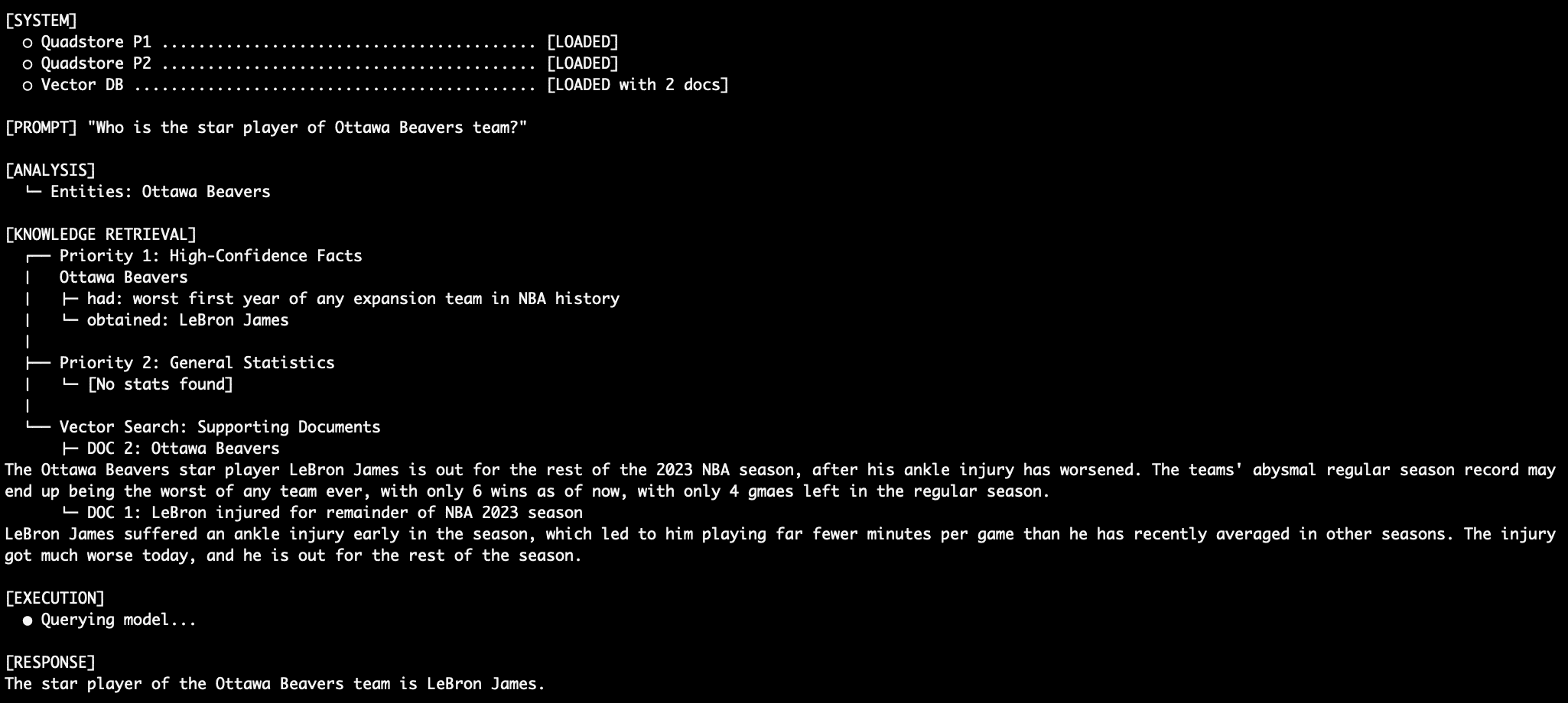
LeBron performs for Ottawa Beavers
As a result of Precedence 1, on this case, explicitly states “Ottawa Beavers obtained LeBron James”, the immediate instructs the LM by no means to complement this with the vector paperwork or statistical abbreviations, thus aiming to eradicate the standard RAG relationship hallucination. The supporting vector database paperwork help this declare as properly, with articles about LeBron and his tenure with the Ottawa NBA workforce. Evaluate this with an LM immediate that dumps conflicting semantic search outcomes right into a mannequin and asks it, generically, to find out which is true.
Question 2: Extra Factual Retrieval
The Ottawa beavers, you say? I’m unfamiliar with them. I assume they play out of Ottawa, however the place, precisely, within the metropolis are they primarily based? Precedence 1 info can inform us. Take into account we’re combating in opposition to what the mannequin itself already is aware of (the Beavers aren’t an precise NBA workforce) in addition to the NBA common stats dataset (which lists nothing concerning the Ottawa Beavers by any means).
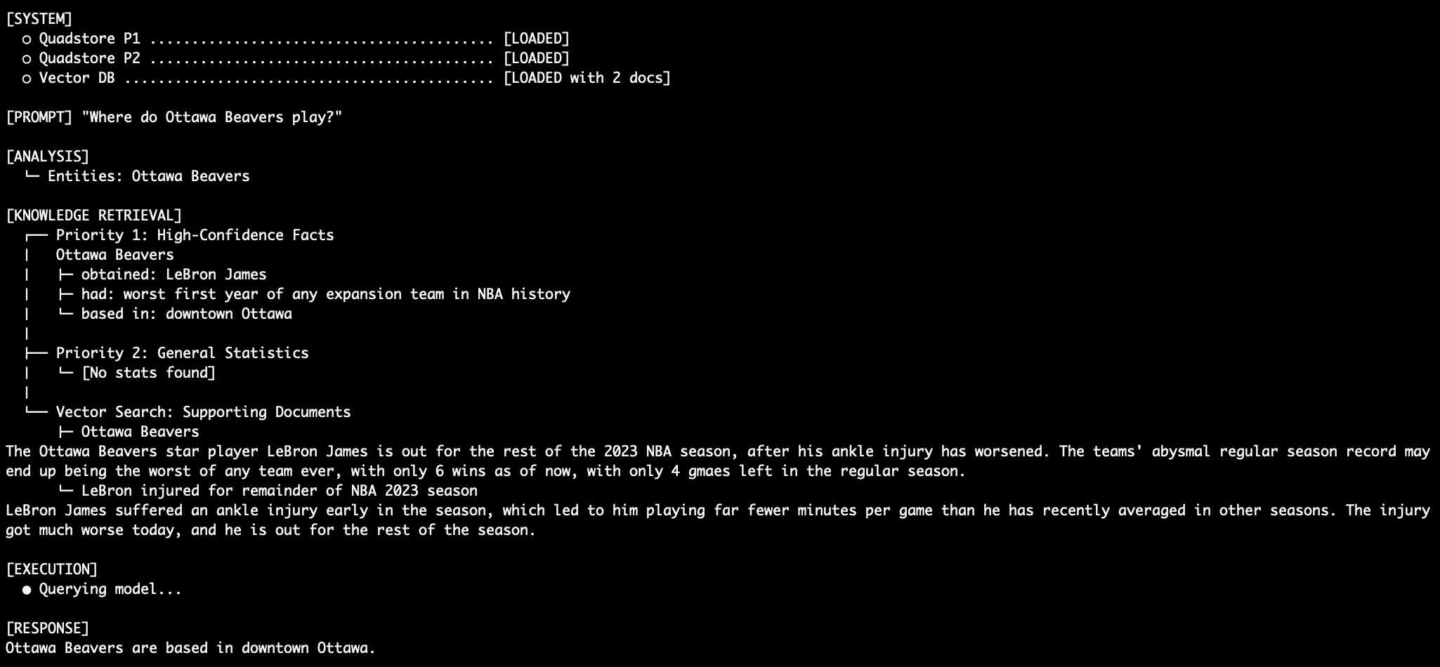
The Ottawa Beavers dwelling
Question 3: Coping with Battle
When querying an attribute in each absolutely the info graph and the final stats graph, akin to “What was LeBron James’ common MPG within the 2023 NBA season?”, the mannequin depends on the Precedence 1 degree knowledge over the prevailing Precedence 2 stats knowledge.
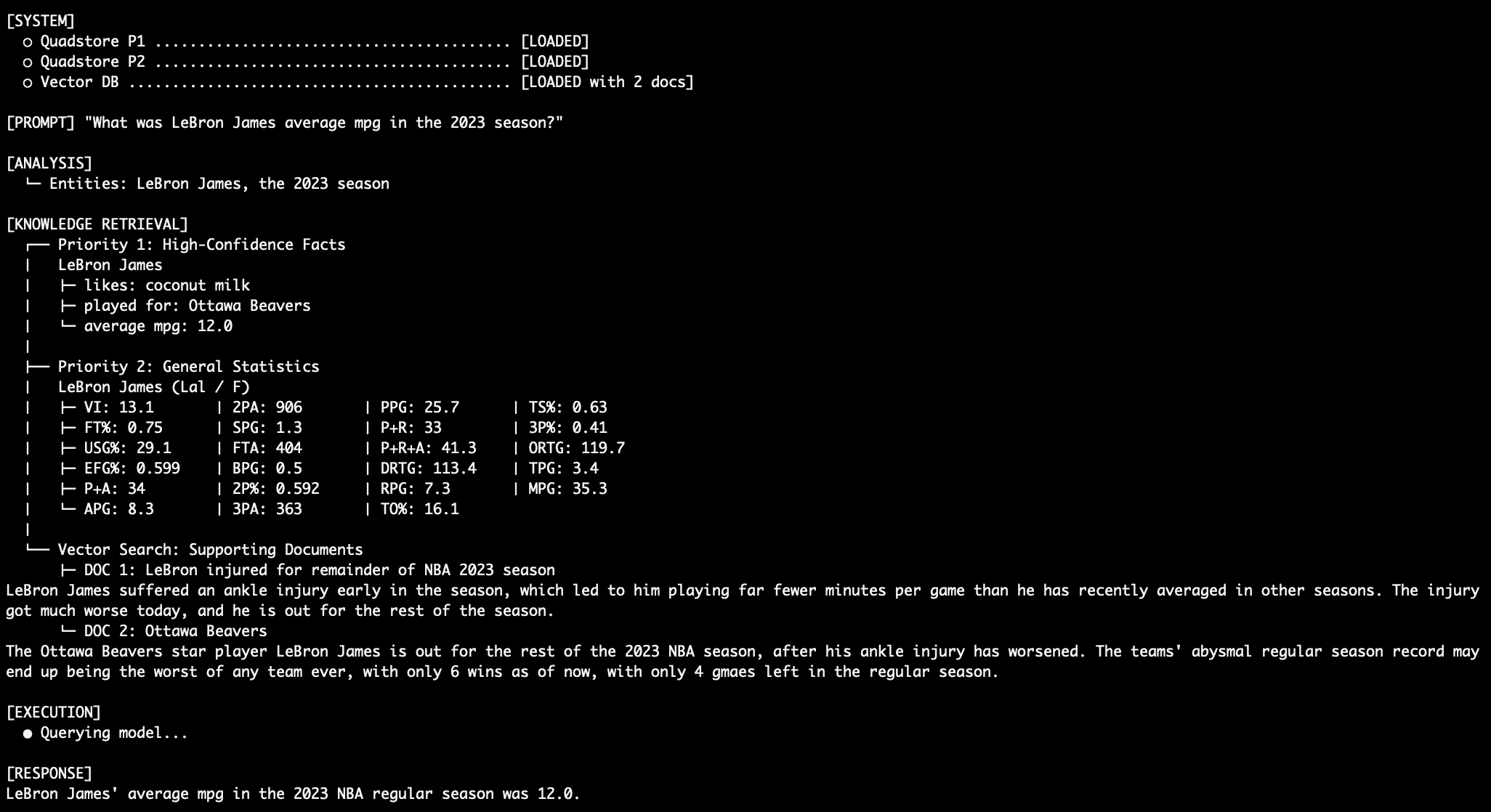
LeBron MPG Question Output
Question 4: Stitching Collectively a Strong Response
What occurs after we ask an unstructured query like “What damage did the Ottawa Beavers star damage endure throughout the 2023 season?” First, the mannequin must know who the Ottawa Beavers star participant is, after which decide what their damage was. That is achieved with a mix of Precedence 1 and Precedence 3 knowledge. The LM merges this easily right into a ultimate response.
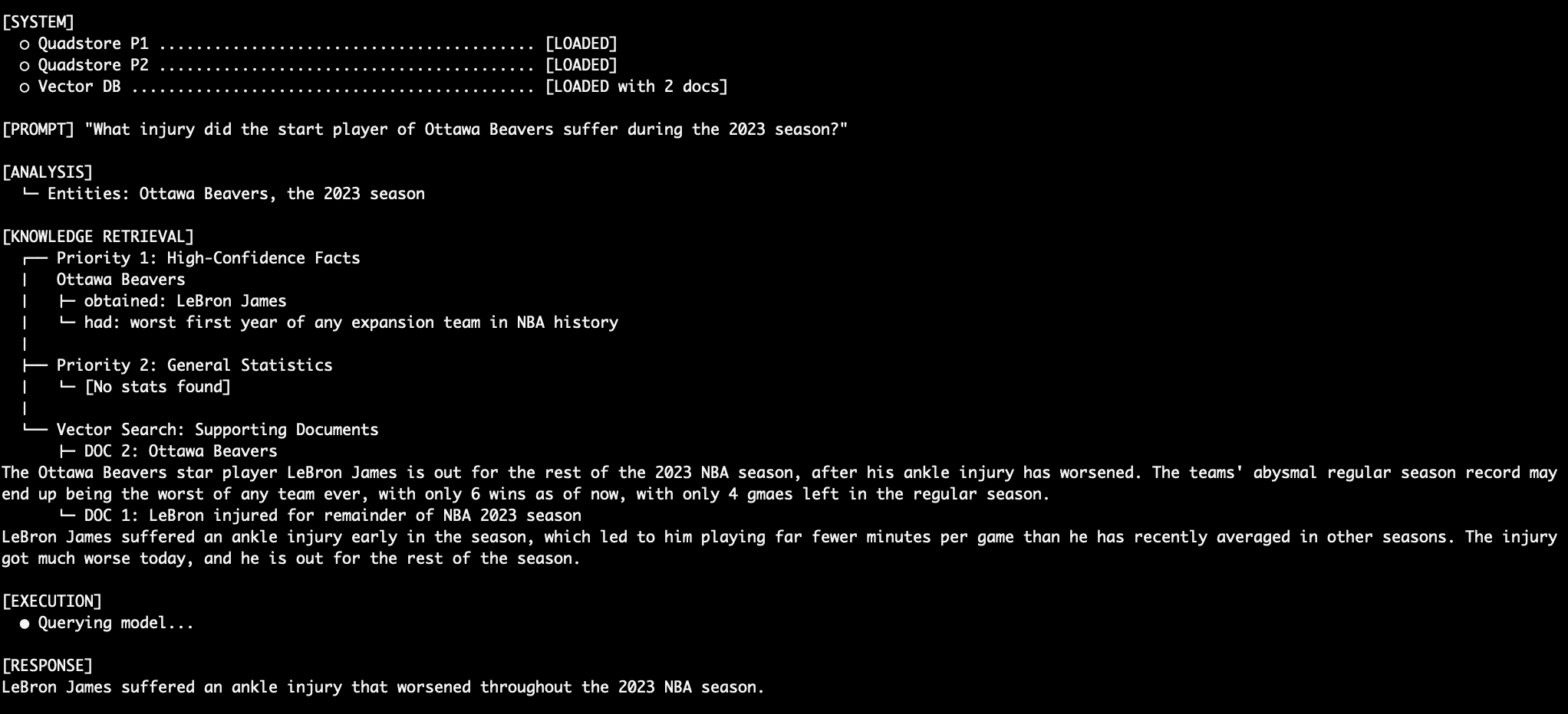
LeBron Damage Question Output
Question 5: One other Strong Response
Right here’s one other instance of sewing collectively a coherent and correct response from multi-level knowledge. “What number of wins did the workforce that LeBron James play for have when he left the season?”
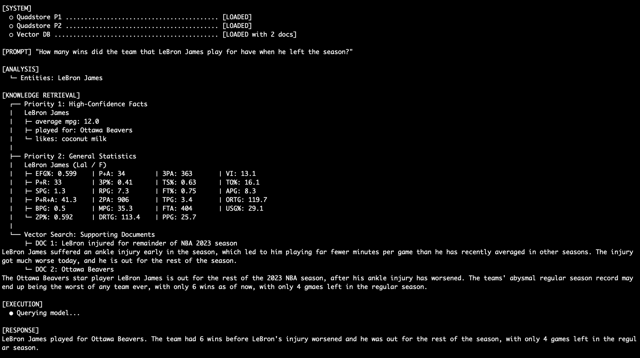
LeBron Damage Question #2 Output
Let’s not overlook that for all of those queries, the mannequin should ignore the truth that conflicting (and inaccurate!) knowledge exists within the Precedence 2 stats graph suggesting (once more, wrongly!) that LeBron James performed for the LA Lakers in 2023. And let’s additionally not overlook that we’re utilizing a easy language mannequin with solely 3 billion parameters (llama3.2:3b).
Conclusion & Commerce-offs
By splitting your retrieval sources into distinct authoritative layers — and dictating actual decision guidelines by way of immediate engineering — the hope is that you simply drastically scale back factual hallucinations, or competitors between in any other case equally-true items of knowledge.
Benefits of this method embrace:
- Predictability: 100% deterministic predictability for crucial info saved in Precedence 1 (objective)
- Explainability: If required, you possibly can drive the LM to output its
[REASONING]chain to validate why Precedence 1 overrode the remaining - Simplicity: No want to coach customized retrieval routers
Commerce-offs of this method embrace:
- Token Overhead: Dumping all three databases into the preliminary context window consumes considerably extra tokens than typical algorithm-filtered retrieval
- Mannequin Reliance: This technique requires a extremely instruction-compliant LM to keep away from falling again into latent training-weight habits
For environments by which excessive precision and low tolerance for errors are necessary, deploying a multi-tiered factual hierarchy alongside your vector database will be the differentiator between prototype and manufacturing.