Information to Propensity Rating Matching (PSM) for Causal Inference

One of many core challenges of knowledge science is drawing significant causal conclusions from observational knowledge. In lots of such circumstances, the purpose is to estimate the true influence of a therapy or behaviour as pretty as doable. This text explores Propensity Rating Matching (PSM), a statistical approach used for that very objective.

In contrast to randomized experiments (A/B checks) or therapy trials, observational research have a tendency to point out preexisting variations between the therapy and management teams which might be necessary. PSM is a statistical mechanism to copy a randomized experiment whereas controlling for confounders.

Allow us to discover it in additional element right here.

Additionally learn: Introduction to Artificial Management Utilizing Propensity Rating Matching

What’s PSM?

Propensity Rating Matching (PSM) is a statistical mechanism to copy a randomized experiment whereas controlling for confounders. This methodology pairs handled and untreated items with related propensity scores, or the chance of receiving the therapy, to kind a well-balanced comparability group.

In 1983, Rosenbaum and Rubin proposed this resolution by describing the propensity rating because the conditional chance of task to a therapy given an noticed set of covariates. PSM tries to cut back biases created by confounders that may distort a easy end result comparability between handled and untreated teams by pairing items with related propensity scores.

Why is PSM Helpful?

Allow us to perceive this with an instance. Suppose we want to discover the affect of a conduct of a buyer, corresponding to going again to a web based store, on an end result, on the choice to make a purchase order. As an alternative of forcing some individuals again, we go for observational knowledge. That is fairly deceptive merely by way of evaluating the acquisition charges of returning vs new prospects, as a result of they’re two vastly completely different cohorts in some ways (corresponding to familiarity with the positioning, shopping behaviors, and so on.).

PSM assists by matching returning prospects to new prospects, matching the identical traits noticed aside from the “returning” standing, and mimicking a randomized managed trial. As soon as the pair is matched, the distinction in buy charges is extra prone to come from the return standing itself.

On this submit, we’ll discover Propensity Rating Matching from idea to Python implementation in depth.

Understanding Propensity Rating Matching

For example the conduct of PSM in motion, we’ll make the most of a publicly accessible e-commerce dataset (On-line Consumers Buying Intention Dataset). The dataset consists of internet session knowledge of an e-commerce system, whether or not the person generated income (buy) in that session (end result), and different options of their shopping conduct. We are going to set up a causal inference state of affairs:

• therapy = if the customer is a returning buyer,
• management = new buyer,
• end result = whether or not the session concludes in a purchase order (Income=True).

We are going to estimate the impact of returning guests on the chance of buy utilizing PSM by matching returning and new guests with related shopping metrics.

A propensity rating is the chance of a unit (corresponding to a person) receiving a therapy given its noticed covariates. In our mannequin, it will be the chance {that a} person is receiving therapy (returning customer), primarily based on their session properties corresponding to pages visited, time spent, and so on. Key assumptions when making causal inference utilizing PSM entail:

1. Conditional Independence: all confounding variables influencing therapy task and impact are noticed and included within the propensity mannequin.
2. Frequent assist (overlap): the chance for any given mixture of covariates just isn’t 0 or 1 (there’s overlap in covariate distributions between handled and management teams). In apply, this interprets to having returning guests and new guests who’ve related properties; if a number of returning guests have very completely different options from new guests that new guests would not have (and vice versa), these must be excluded, or PSM won’t be helpful.

PSM Workflow

The overall PSM workflow is:

• Propensity rating estimation – sometimes match a logistic regression of Therapy ~ Covariates to get every unit’s propensity
• Matching – pair every handled unit with a number of management items having shut propensity scores
• Steadiness diagnostics – verify if the matched samples have balanced covariates.
  (If the imbalance stays, refine the mannequin or the matching methodology)
• Therapy impact estimation – compute the end result distinction between matched handled and management teams

Case Examine Setup: E-commerce Dataset and Therapy State of affairs

On this sensible state of affairs, we additional make the most of the On-line Consumers Buying Intention dataset from the UCI Machine Studying Repository. This dataset incorporates 12,330 retail web site periods, and about 15% of periods finish with a purchase order (Income=True). Every session has the data such because the variety of completely different pages visited (Administrative, Informational, ProductRelated), the quantity spent on these pages, bounce charge, exit charge, web page worth, big day indicator (how near a vacation), and a few categorical options (Month, Browser, Area, TrafficType, VisitorType, and Weekend).

Described therapy

We decide therapy = 1 (for “Returning_Visitor”) and 0 (for “New_Visitor”) primarily based on VisitorType. Round 85% of periods are attended by customers returning to the service. Subsequently, the group is significantly bigger than that of the management.

Final result

The Income characteristic is True if the session resulted in a purchase order (conversion) or False if no buy occurred. By factoring in conduct, we need to estimate how way more possible the acquisition is for repeat prospects as a result of they’re repeat prospects. Whereas returning guests are logging on at a a lot greater uncooked conversion charge than new guests, additionally they examine extra merchandise and keep on the positioning longer. We are going to use PSM to match return vs. new guests by controlling for these elements.

Let’s load the dataset and do some gentle preprocessing for our evaluation. We’ll use pandas to load the CSV after which encode the related columns for our binary therapy and end result:

import pandas as pd

# Load the dataset
Df = pd.read_csv("online_shoppers_intention.csv")


# Encode categorical variables of curiosity
Df['Revenue'] = df['Revenue'].map({False: 0, True: 1})

Df['Treatment'] = df['VisitorType'].map({"Returning_Visitor": 1, "New_Visitor": 0})

# (Drop or mix ‘Different’ customer sorts if current, for simplicity)
Df = df[df['VisitorType'].isin(["Returning_Visitor", "New_Visitor"])]


# Take a fast take a look at therapy vs end result charges
Print(pd.crosstab(df['Treatment'], df['Revenue'], normalize="index") * 100)

Within the above, we create a brand new column Therapy, which is 1 for returning guests and 0 for brand spanking new guests. The crosstab will present the acquisition charge (% Income=1) for every group earlier than matching. We anticipate returning guests to have a better conversion charge than new guests initially. Nonetheless, this uncooked distinction is confounded by different variables. To isolate the impact of being a return customer, we proceed to estimate propensity scores.

Propensity Rating Estimation (Logistic Regression)

For this, we’ll estimate every session’s propensity rating (chance of being a returning customer) given its noticed options. We are going to use a logistic regression mannequin for this train. The covariates ought to embody all elements that affect the chance of being a returning customer and are associated to the end result. In our case, believable covariates are the varied web page go to counts, durations, and metrics like bounce charge, and so on., since returning guests doubtless have completely different shopping behaviors. We embody a broad set of options from the session (excluding any which might be trivial or happen after the choice to return). For simplicity, let’s use the numeric options accessible:

from sklearn.linear_model import LogisticRegression

# Options to make use of for propensity mannequin (all numerical besides goal)
Covariates = ['Administrative', 'Administrative_Duration', 'Informational',
              'Informational_Duration', 'ProductRelated', 'ProductRelated_Duration',
              'BounceRates', 'ExitRates', 'PageValues', 'SpecialDay']

X = df[covariates]

T = df['Treatment']


# Match logistic regression to foretell Therapy
Ps_model = LogisticRegression(solver="lbfgs", max_iter=1000)

Ps_model.match(X, T)


# Predicted propensity scores:
Propensity_scores = ps_model.predict_proba(X)[:, 1]

Df['PropensityScore'] = propensity_scores

Print(df[['Treatment', 'PropensityScore']].head(10))

Right here we practice a logistic regression the place the dependent variable is Therapy (returning vs new) and the impartial variables are the session options. Every session will get a PropensityScore between 0 and 1. A excessive rating (near 1) means the mannequin thinks this session appears very very similar to a returning customer primarily based on the shopping traits; a rating close to 0 means it appears like a brand new customer profile.

Visualising Propensity Rating Distributions

After becoming, it’s good apply to visualise the propensity rating distributions for handled and management teams to verify overlap (the positivity assumption). Ideally, there must be substantial overlap; if the distributions hardly overlap, PSM will not be dependable as a result of we lack comparable counterparts.

Beneath is a distribution plot of propensity scores for the 2 teams:

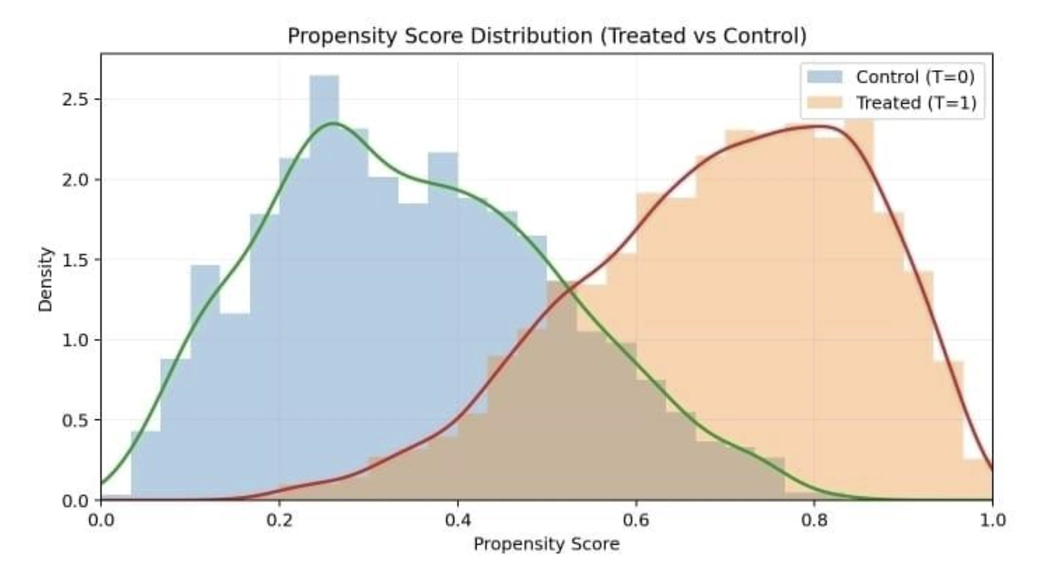
Propensity rating distribution for handled (returning guests) and untreated (new guests). We see some overlap on this case, which is considerably important for a legitimate match.

In our state of affairs, we anticipate returning guests on common to have greater propensity scores (since they’re returners), but when many new guests have moderate-to-high scores and a few returners have decrease scores, we’ve got overlap. If there have been returners with extraordinarily excessive scores >0.9 and no new guests in that vary, these returners can be exhausting to match and may have to be dropped (frequent assist problem).

Matching: Pairing on Propensity Scores

With propensity scores in hand, we proceed to match every handled unit with a number of management items with related scores. A easy and generally used methodology is one-to-one nearest neighbor matching with out alternative: for every handled unit, discover the management unit with the closest propensity rating, and don’t reuse management items as soon as matched. This yields a matched pattern of handled and management items of equal dimension. Different methods embody many-to-one matching, caliper (tolerance for optimum distance allowed) matching, optimum matching, and so on.. For this demonstration, we’ll use one-to-one nearest neighbor matching.

We are able to carry out matching manually or utilizing libraries. Beneath is the best way to do one-to-one matching in Python utilizing a nearest neighbors’ strategy from scikit-learn:

import numpy as np
from sklearn.neighbors import NearestNeighbors

# Break up the info into handled and management dataframes
Treated_df = df[df['Treatment'] == 1].copy()

Control_df = df[df['Treatment'] == 0].copy()


# Use nearest neighbor on propensity rating
Nn = NearestNeighbors(n_neighbors=1, metric="euclidean")

nn.match(control_df[['PropensityScore']])

distances, indices = nn.kneighbors(treated_df[['PropensityScore']])


# `indices` provides index of closest management for every handled
Matched_pairs = record(zip(treated_df.index, control_df.iloc[indices.flatten()].index))

Print(f"Matched {len(matched_pairs)} pairs")

We match a nearest neighbors mannequin on the management group’s propensity scores, then for every handled remark, discover the closest management. The end result matched_pairs is a listing of (treated_index, control_index) pairs of matched observations. We must always get roughly as many pairs as the scale of the smaller group, right here the management group, as a result of as soon as we exhaust the controls, we can not match the remaining handled items with out reuse. If the dataset has extra handled than management items, as in our case, some handled items will stay unmatched. In apply, analysts typically drop these unmatched handled items and focus the evaluation on the area of frequent assist.

After matching, we create a brand new DataFrame for the matched pattern containing solely the matched handled and matched management observations. This matched pattern is what we’ll use to estimate the therapy impact. However first, did matching reach balancing the covariates?

Steadiness Diagnostics

An necessary process in PSM evaluation is to verify whether or not or not the handled and management teams are certainly extra balanced after matching. We illustrate and evaluate the distributions for the covariates of every matched handled vs matched management. To make it extra handy, we are able to observe the SMD of every covariate earlier than and after matching is full. SMD measures the distinction in means between teams divided by the pooled customary deviation. It’s a unitless measure of imbalance, the place an SMD of 0 signifies excellent steadiness. A typical rule of thumb treats an absolute SMD under 0.1 as a negligible imbalance.

Let’s compute and evaluate SMDs for just a few key options earlier than and after matching:

# Operate to compute standardized imply distinction
def standardized_diff(x, group):
    # x: sequence of covariate, group: sequence of Therapy (1/0)
    Treated_vals = x[group == 1]
    Control_vals = x[group == 0]

    Mt, mc = treated_vals.imply(), control_vals.imply()
    Var_t, var_c = treated_vals.var(), control_vals.var()

    Return (mt - mc) / np.sqrt((var_t + var_c) / 2)


Covariates_to_check = ['ProductRelated', 'ProductRelated_Duration', 'BounceRates']

For cov in covariates_to_check:
    Smd_before = standardized_diff(df[cov], df['Treatment'])

    Smd_after = standardized_diff(treated_df.loc[[i for i, _ in matched_pairs], cov],
                                  Control_df.loc[[j for _, j in matched_pairs], cov])

    Print(f"{cov}: SMD earlier than = {smd_before:.3f}, after = {smd_after:.3f}")

Output

This can output one thing like (for instance):

ProductRelated: SMD earlier than = 0.28, after = 0.05

ProductRelated_Duration: SMD earlier than = 0.30, after = 0.08

BounceRates: SMD earlier than = -0.22, after = -0.04

The precise values will change with the info, however we anticipate that SMDs shrink considerably in direction of 0 after matching. Be aware that the variety of product-related pages (ProductRelated), for instance, had a reasonably massive imbalance earlier than (the handled customers seen, on common, extra pages than controls, SMD 0.28) and decreased to 0.05 after matching – suggesting a profitable balancing impact. The identical advantages are noticed for complete product web page period and bounce charge. That tells us our propensity mannequin plus matching did an affordable job of producing related teams. If, actually, there’s any covariate that also has a excessive SMD (say > 0.1) after a match, one might contemplate refining the propensity mannequin (assume interplay phrases or non-linear phrases, and so on.) or imposing a caliper to power a more in-depth match.

The determine under illustrates the covariate steadiness earlier than and after matching for our instance (with absolute SMDs for just a few covariates):

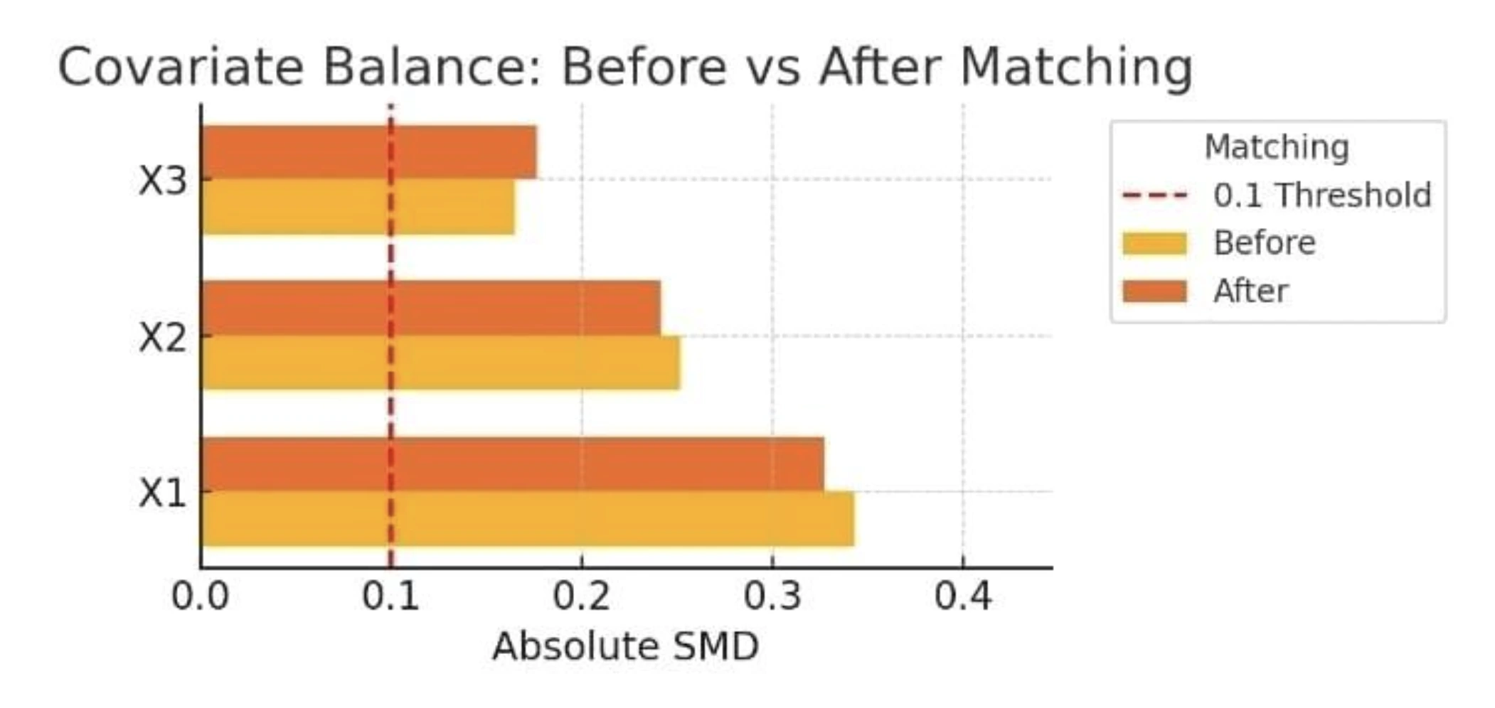
Covariate steadiness earlier than and after matching. The bar chart shows absolute standardized imply variations for 3 pattern options. After matching, the steadiness improves, the bars turn into considerably smaller, and all covariate variations fall under the 0.1 threshold (crimson dashed line), indicating negligible imbalance. What we see is that PSM has made the handled and management teams way more related when it comes to the noticed variables. Now we are able to evaluate these related matched teams primarily based on the outcomes to evaluate the causal impact.

Estimating the Causal Impact

Lastly, we compute the therapy impact on the end result with the matched pattern. With one-to-one matched pairs, our reply for a binary end result is that we are able to evaluate the common conversion of handled vs. management outcomes within the matched pattern. This gives an estimate of the Common Therapy Impact on the Handled (ATT) – the distinction in buy chance for returning guests if they’d as an alternative been new guests (counterfactually).

On the situation, if after matching we’ve got the next numbers: Returning guests buy charge is 12.5 per cent, new guests buy charge = 10 per cent. The ATT can be 2.5 share factors (0.125 – 0.100). This suggests that being a returning customer causally will increase the acquisition chance by 2.5 factors (if our assumptions maintain).

In code, that is simply:

matched_treated_indices = [i for i, _ in matched_pairs]
matched_control_indices = [j for _, j in matched_pairs]

att = df.loc[matched_treated_indices, 'Revenue'].imply() - 
      df.loc[matched_control_indices, 'Revenue'].imply()

print(f"ATT (therapy impact on buy charge) = {att*100:.2f} share factors")

Be aware that this estimate is restricted to the inhabitants of returning guests (ATT). We would want a little bit of a distinct evaluation (and perhaps weighting) if we wished the common therapy impact in the entire inhabitants (ATE). In quite a few circumstances, ATT is a key problem: “how a lot did the therapy assist those that obtained it?” In our case, we’re measuring how a lot greater the conversion is for returning customers on account of their returning standing reasonably than behavioral variations.

Deciphering the end result

If the ATT is optimistic (say 2.5pp, as was the case in our supposed end result), which means returning guests usually tend to buy not just by viewing extra pages or spending extra time (and we managed for these), however on account of being a return buyer (e.g., extra belief, intent). If the ATT is nearly zero, the noticed covariates clarify your entire distinction in uncooked buy charges, and returning standing itself provides no additional enhance as soon as we account for them.

Lastly, it’s important to acknowledge limitations in PSM. PSM can solely measure noticed confounding results within the knowledge. Furthermore, poor overlap or a mis-specified propensity mannequin can even trigger inaccurate estimates. Sensitivity analyses strengthen the evaluation, and researchers can use different strategies. For example, inverse chance weighting or doubly sturdy estimation can be utilized to verify robustness.

Conclusion

Propensity Rating Matching just isn’t so new to the knowledge scientist, and is an extremely highly effective approach for causal inference with observational knowledge. On this weblog, we defined how PSM works in idea and apply utilizing an e-commerce case examine. We exhibit estimation of propensity scores with a logistic regression, match therapy and management items with related scores, verify covariate steadiness with diagnostics like standardized imply variations, and estimate the causal impact on an end result. By matching returning guests with new guests who behaved equally on a web based procuring website, we might seize the position of being a returning customer in figuring out buy chance.

Our evaluation confirmed that returning guests do certainly have (even after accounting for his or her shopping conduct) a greater conversion chance.

The method we adopted – Introduction → Propensity Mannequin → Matching → Analysis → Impact Estimation.

After we use PSM, we’d like to pay attention to the choice of covariates (we should contemplate all related confounders), assumptions (overlap between propensity scores), and understand that PSM minimizes bias from noticed covariates however doesn’t take away bias from hidden covariates. Contemplating this, PSM gives an sincere and clear methodology to approximate a trial and infer causality out of your knowledge.

Dharmateja Priyadarshi Uddandarao is a knowledge scientist and statistician who at the moment serves as a Senior Information Scientist–Statistician at Amazon. He has led tasks at main know-how corporations, together with Capital One and Amazon, making use of advanced analytical methods to deal with real-world challenges.